
Customize Your Interactive EDA: Explore the Fuel Economy of the U.S. Car Market
Interactive EDA is nice but customized interactive EDA is even nicer. To celebrate the new CRAN version of my ‘ExPanDaR’ package I prepare a customized variant of ‘ExPanD’ to explore the U.S. EPA data on fuel economy. Our objective is to develop an interactive display that guides the reader on how to explore the fuel economy data in an intuitive way.
First, let’s load the packages and the data from EPA’s web page. In addition, I prepared a small data set containing the countries of domicile for the car producers with more than 100 different cars listed in the EPA data (covering the vast majority of the EPA sample).
library(tidyverse)
library(ExPanDaR)

# The following two chuncks borrow
# from the raw data code of the
# fueleconomy package by Hadley Wickham,
# See: https://github.com/hadley/fueleconomy

if(!file.exists("vehicles.csv")) {
  tmp <- tempfile(fileext = ".zip")
  download.file("http://www.fueleconomy.gov/feg/epadata/vehicles.csv.zip",
                tmp, quiet = TRUE)
  unzip(tmp, exdir = ".")
}

raw <- read.csv("vehicles.csv", stringsAsFactors = FALSE)
countries <- read.csv("https://joachim-gassen.github.io/data/countries.csv",
                      stringsAsFactors = FALSE)
Next, I merge the data and re-code some factors to be more stable across time as the EDA has made several coding changes over time.
vehicles <- raw %>%
  mutate(car = paste(make, model, trany),
         mpg_hwy = ifelse(highway08U > 0, highway08U, highway08),
         mpg_city = ifelse(city08U > 0, city08U, city08)) %>%
  left_join(countries) %>%
  select(car, make, country, trans = trany,
         year,
         class = VClass, drive = drive, fuel = fuelType,
         cyl = cylinders, displ = displ,
         mpg_hwy, mpg_city) %>%
  filter(drive != "",
         year > 1985,
         year < 2020) %>%
  mutate(fuel = case_when(
   fuel == "CNG" ~ "gas",
   fuel == "Gasoline or natural gas" ~ "hybrid_gas",
   fuel == "Gasoline or propane" ~ "hybrid_gas",
   fuel == "Premium and Electricity" ~ "hybrid_electro",
   fuel == "Premium Gas or Electricity" ~ "hybrid_electro",
   fuel == "Premium Gas and Electricity" ~ "hybrid_electro",
   fuel == "Regular Gas or Electricity" ~ "hybrid_electro",
   fuel == "Electricity" ~ "electro",
   fuel == "Diesel" ~ "diesel",
   TRUE ~ "gasoline"
  ),
  class = case_when(
    grepl("Midsize", class) ~ "Normal, mid-size",
    grepl("Compact", class) ~ "Normal, compact",
    grepl("Small Station Wagons", class) ~ "Normal, compact",
    grepl("Large Cars", class) ~ "Normal, large",
    grepl("Minicompact", class) ~ "Normal, sub-compact",
    grepl("Subcompact", class) ~ "Normal, sub-compact",
    grepl("Two Seaters", class) ~ "Two Seaters",
    grepl("Pickup Trucks", class) ~ "Pickups",
    grepl("Sport Utility Vehicle", class) ~ "SUVs",
    grepl("Special Purpose Vehicle", class) ~ "SUVs",
    grepl("Minivan", class) ~ "(Mini)vans",
    grepl("Vans", class) ~ "(Mini)vans"
  ),
  drive = case_when(
    grepl("4-Wheel", drive) ~ "4-Wheel Drive",
    grepl("4-Wheel", drive) ~ "4-Wheel Drive",
    grepl("All-Wheel", drive) ~ "4-Wheel Drive",
    grepl("Front-Wheel", drive) ~ "Front-Wheel Drive",
    grepl("Rear-Wheel", drive) ~ "Rear-Wheel Drive"
  ),
  trans = case_when(
    grepl("Automatic", trans) ~ "Automatic",
    grepl("Manual", trans) ~ "Manual"
  )) %>%
  na.omit()
Now, the EPA fuel economy data is ready for exploration. Nothing stops you from firing up ‘ExPanD’ right away.
ExPanD(vehicles, cs_id = "cars", ts_id = "year")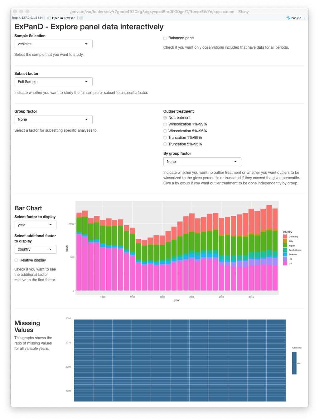
ExPanD with fuel economy data, standard look
This works but the display is not optimal for what we are after. It includes components that are not needed (e.g., the missing values display as the data do not contain any missing observations) and lacks documentation. We can do better by using some of the new customization features of the ‘ExPanD’ app. See below for a ‘customized’ version that guides the reader a little bit better through the analysis by omitting unneeded displays, adding variable definitions, setting informative defaults and adding explanatory texts between displays.
df_def <- data.frame(
  var_name = names(vehicles),
  var_def = c("Make, model and transition type indentifying a unique car in the data",
              "Make of car",
              "Country where car producing firm is loacted",
              "Transition type (automatic or manual)",
              "Year of data",
              "Classification type of car (simplified from orginal data)",
              "Drive type of car (Front Wheel, Rear Wheel or 4 Wheel)",
              "Fuel type (simplified from orginal data)",
              "Number of engine cylinders",
              "Engine displacement in liters",
              "Highway miles per gallon (MPG). For electric and CNG vehicles this number is MPGe (gasoline equivalent miles per gallon).",
              "City miles per gallon (MPG). For electric and CNG vehicles this number is MPGe (gasoline equivalent miles per gallon)."),
  type = c("cs_id", rep("factor", 3), "ts_id", rep("factor", 3), rep("numeric", 4))
)

html_blocks <- c(
  paste("<div class='col-sm-12'>",
        "By default, this display uses all data from car makes with more",
        "than 100 cars in the 'fueleconomy.gov' database.",
        "Above, you can limit the analysis to cars from a certain make,",
        "class, country, fuel type or other factor present in the data.",
        "</div>"),
  paste("<div class='col-sm-12'>",
        "In the display above, remove the check mark to see the absolute",
        "number of cars included in the data each year.",
        "Also, change the additional factor to see how the distribution",
        "of cars across countries, transition types, etc. changes over time",
        "</div>"),
  paste("<div class='col-sm-12'>",
        "In the two tables above, you can assess the distributions of the",
        "four numerical variables of the data set. Which car has the",
        "largest engine of all times?",
        "</div>"),
  paste("<div class='col-sm-12'>",
        "Explore the numerical variables across factors. You will see,",
        "not surprisingly, that fuel economy varies by car class.",
        "Does it also vary by drive type?",
        "</div>"),
  paste("<div class='col-sm-12'>",
        "The above two panels contain good news. Fuel economy has",
        "increased over the last ten years. See for yourself:",
        "Has the size of engines changed as well?",
        "</div>"),
  paste("<div class='col-sm-12'>",
        "The scatter plot documents a clear link between engine size",
        "and fuel economy in term of miles per gallon.",
        "Below, you can start testing for associations.",
        "</div>"),
  paste("<div class='col-sm-12'>",
        "Probably, you will want to test for some associations that",
        "require you to construct new variables. No problem. Just enter the",
        "variable definitions above. Some ideas on what to do:",
        "<ul><li>Define country dummies (e.g., country == 'US') to see",
        "whether cars from certain countries are less fuel efficient than others.</li>",
        "<li>Define a dummy for 4-Wheel drive cars to assess the penalty",
        "of 4-Wheel drives on fuel economy.</li>",
        "<li>If you are from a metric country, maybe your are mildly annoyed",
        "by the uncommon way to assess fuel economy via miles per gallon.",
        "Fix this by defining a liter by 100 km measure",
        "(hint: 'l100km_hwy := 235.215/mpg_hwy').</li></ul>",
        "</div>"),
  paste("<div class='col-sm-12'>",
        "Above, you can play around with certain regression parameters.",
        "See how robust coefficients are across car classes by estimating",
        "the models by car class ('subset' option).",
        "Try a by year regression to assess the development of fuel economy",
        "over time. <br> <br>",
        "If you like your analysis, you can download the configuration",
        "and reload it at a later stage using the buttons below.",
        "</div>")
)

cl <- list(
  ext_obs_period_by = "2019",
  bgbg_var = "mpg_hwy",
  bgvg_var = "mpg_hwy",
  scatter_loess = FALSE,
  delvars = NULL,
  scatter_size = "cyl",
  bar_chart_relative = TRUE,
  reg_x = c("cyl", "displ", "trans"),
  scatter_x = "displ",
  reg_y = "mpg_hwy",
  scatter_y = "mpg_hwy",
  bgvg_byvar = "class",
  quantile_trend_graph_var = "mpg_hwy",
  bgbg_byvar = "country",
  scatter_color = "country", bar_chart_var2 = "class",
  ext_obs_var = "mpg_hwy",
  trend_graph_var1 = "mpg_hwy",
  trend_graph_var2 = "mpg_city",
  sample = "vehicles"
)

ExPanD(vehicles, df_def = df_def, config_list = cl,
       title = "Explore the Fuel Economy of Cars in the U.S. Market",
       abstract = paste("This interactive display features the <a href=https://www.fueleconomy.gov/>",
                        "fuel economy data provided by the U.S. Environmental Protection Agency</a>",
                        "and allows you to explore the fuel economy of cars in the U.S. market",
                        "across time and other dimensions. Scroll down and enjoy!"),
       components = c(subset_factor = TRUE,
                      html_block = TRUE,
                      bar_chart = TRUE,
                      html_block = TRUE,
                      descriptive_table = TRUE,
                      ext_obs = TRUE,
                      html_block = TRUE,
                      by_group_bar_graph = TRUE,
                      by_group_violin_graph = TRUE,
                      html_block = TRUE,
                      trend_graph = TRUE,
                      quantile_trend_graph = TRUE,
                      html_block = TRUE,
                      scatter_plot = TRUE,
                      html_block = TRUE,
                      udvars = TRUE,
                      html_block = TRUE,
                      regression = TRUE,
                      html_block = TRUE),
       html_blocks = html_blocks
)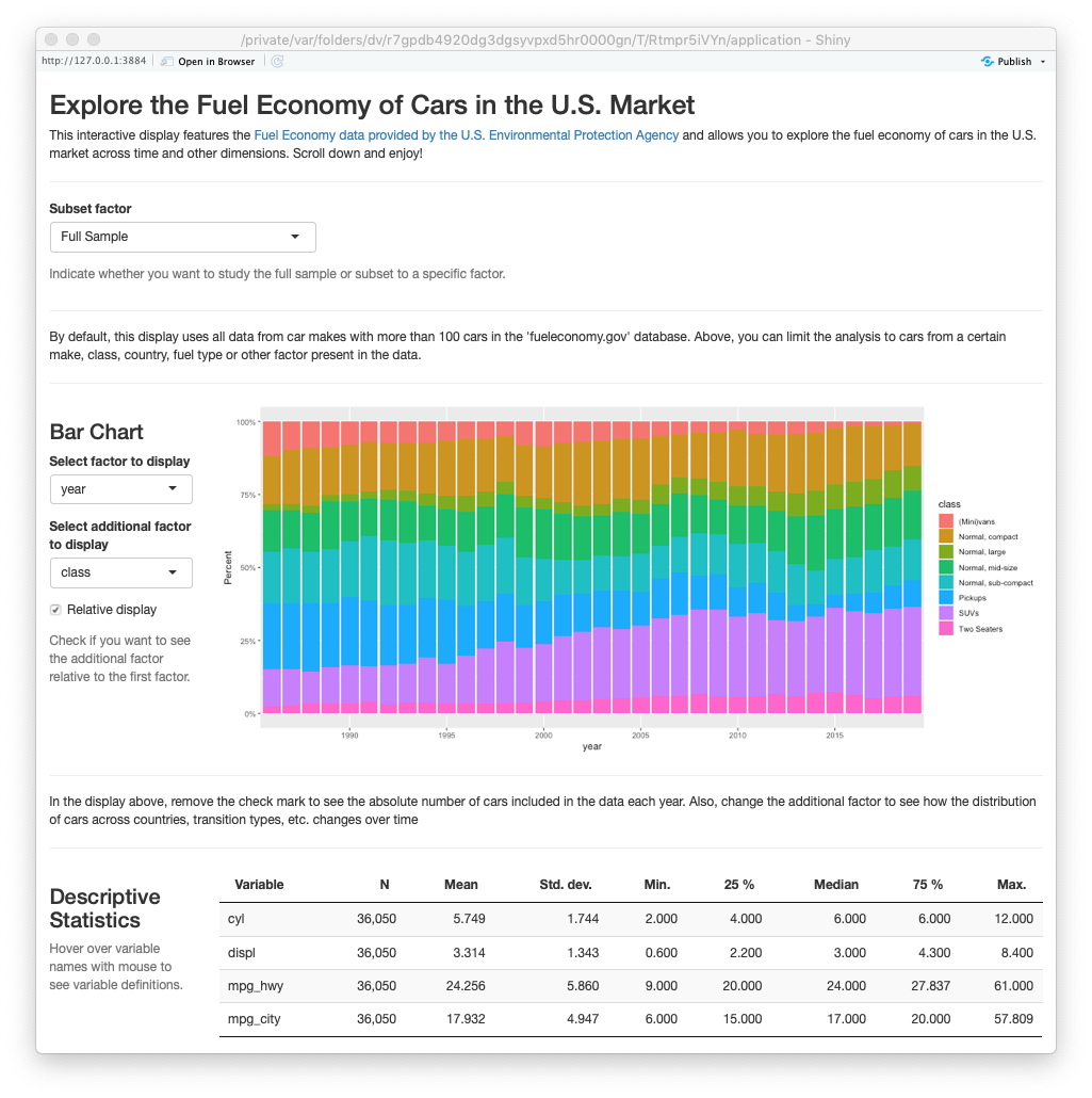
ExPanD with fuel economy data, customized look
You can assess the customized EDA online here. While customizing ‘ExPanD’ requires extra work, it helps to make the EDA flow better. Fur further information on how to build customized EDAs using ‘ExPanD’ step-by-step, please refer to the new vignette of the package.
Feel free to comment below. Alternatively, you can reach me via email or twitter.
Enjoy!

