
Using the ExPanDaR package for panel data exploration
Did you ever want to do a quick exploratory pass on a panel data set? Did you ever wish to give somebody (e.g., a reviewer or a fellow researcher), the opportunity to explore your data and your findings but can’t provide your raw data? Do you get bored from producing the same tables and figures over and over again for your panel data project? If your answer to one of the questions above is yes, then the new ExPanDaR R package might be worth a look.
ExPanDaR does two things:
It provides the code base for the ExPanD web app. ExPanD is a shiny based app supporting interactive exploratory data analysis. See here for an online version presenting the same data that we will explore below.
It provides a set of functions that I hope is useful for a panel data exploration workflow and prepares output that you would include into a typical applied panel data study.
To see what ExPanDaR has to offer, let’s take a quick tour. For more detailed guidance on how to use a specific function presented below, take a look at the package documentation.
Data Preparation
ExPanDaR expects the data to be organized in long format. This implies that each observation (a row) is identified by cross-sectional and time series identifiers and that variables are organized by columns. While you can have a vector of variables jointly determining the cross-section, the time-series needs to be identified by a unique sortable variable. The ExPanDaR functions treat cross-sectional identifiers as factors and expect the time-series identifier to be coercible into an ordered factor.
For this walk-through I will use the data set russell_3000, which comes with the package. It contains some financial reporting and stock return data of Russell 3000 firms and has been collected from Google Finance and Yahoo Finance using the tidyquant package in the summer of 2017. A word of caution: While the data appears to be relatively decent quality I would advise against using this data for scientific work without verifying its integrity first. These are the variables included in the data.
| Variable | Definition |
|---|---|
| coid | Company identifier |
| period | Fiscal year |
| coname | Company name |
| sector | Sector |
| industry | Industry |
| toas | Total assets at period end (M US-$) |
| sales | Sales of the period (M US-$) |
| equity | Total equity at period end (M US-$) |
| debt_ta | Total debt (% total assets) |
| eq_ta | Total equity (% total assets) |
| gw_ta | Goodwill (% total assets) |
| oint_ta | Other intangible assets (% total assets) |
| ppe_ta | Property, plant and equipment (% total assets) |
| ca_ta | Current assets (% total assets) |
| cash_ta | Cash (% total assets) |
| roe | Return on equity (net income divided by average equity) |
| roa | Return on assets (earnings before interest and taxes divided by average equity) |
| nioa | Net income divided by average assets |
| cfoa | Cash flow from operations divided by average assets |
| accoa | Total accruals divided by average assets |
| cogs_sales | Cost of goods sold divided by sales |
| ebit_sales | Earnings before interest and taxes divided by sales |
| ni_sales | Net income divided by sales |
| return | Stock return of the period (%) |
Let’s see whether coid and period identify a panel observation.
any(duplicated(russell_3000[,c("coid", "period")]))## [1] FALSEThis seems to be the case.
Now you can start exploring the data interactively. The code
ExPanD(df = russell_3000, df_def = russell_3000_data_def,
       config_list = ExPanD_config_russell_3000,
       abstract = "Data is from Google Finance and Yahoo Finance.")
will start the ExPanD app (online instance can be found here).
But in this blog post I want to showcase the functions of the ExPanDaR package. So, as a first step, let’s use ExPanDaR’s function prepare_missing_values_graph() to eyeball how frequently observations are missing in the data set.
prepare_missing_values_graph(russell_3000, ts_id = "period")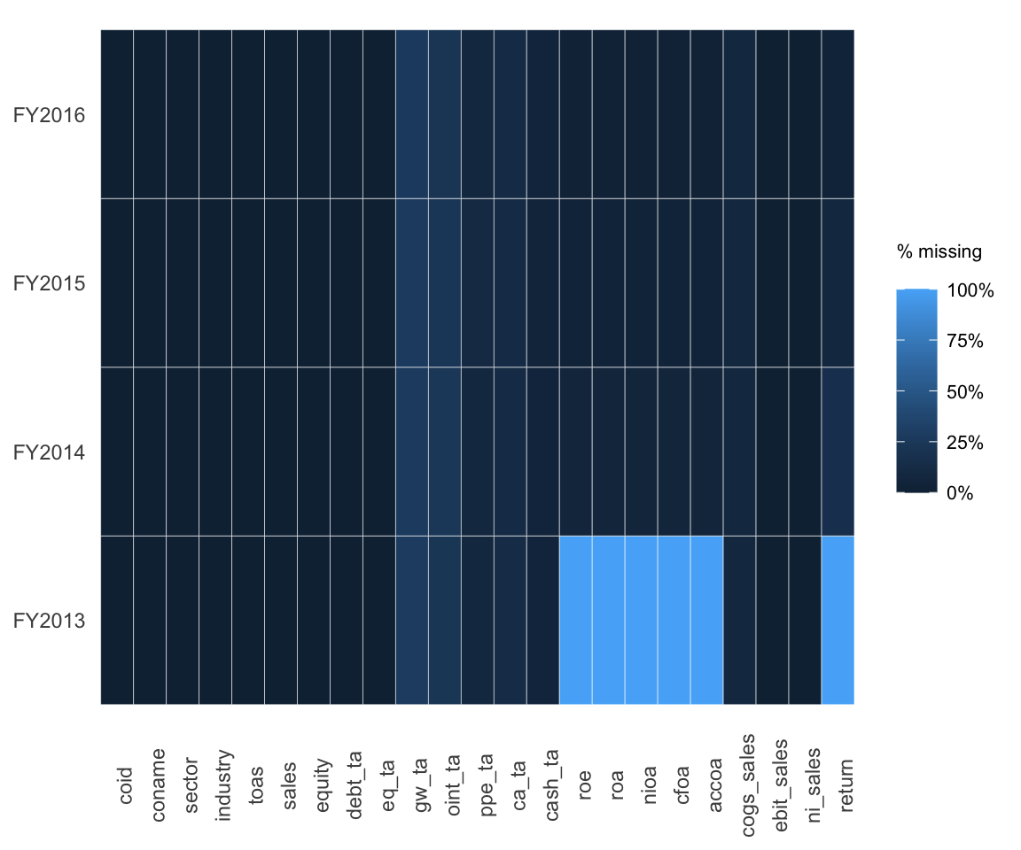
OK. This does not look too bad. Only FY2013 seems odd, as some variables are completely missing. Guess why? They are calculated using lagged values of total assets. So, in the following, let’s focus on some profitability measures and on the fiscal years 2014 to 2016 (a short panel, I know). Time to check the descriptive statistics using the prepare_descriptive_table() function.
r3 <- droplevels(russell_3000[russell_3000$period > "FY2013",
                              c("coid", "coname", "period", "sector", "toas",
                                "nioa", "cfoa", "accoa", "return")])
t <- prepare_descriptive_table(r3)
t$kable_ret  %>%
kable_styling("condensed", full_width = F, position = "center")| N | Mean | Std. dev. | Min. | 25 % | Median | 75 % | Max. | |
|---|---|---|---|---|---|---|---|---|
| toas | 6,643 | 8,722.510 | 35,846.713 | 0.800 | 463.225 | 1,600.050 | 5,100.500 | 861,395.000 |
| nioa | 6,399 | 0.001 | 0.096 | -2.692 | -0.002 | 0.017 | 0.037 | 0.463 |
| cfoa | 6,399 | 0.033 | 0.084 | -2.121 | 0.021 | 0.041 | 0.065 | 0.460 |
| accoa | 6,399 | -0.032 | 0.052 | -0.712 | -0.046 | -0.026 | -0.012 | 0.621 |
| return | 6,009 | 0.097 | 0.433 | -0.938 | -0.136 | 0.065 | 0.269 | 6.346 |
Take a look at the minima and the maxima of some of the variables (e.g., net income over assets (nioa)). Normally, it should be around -50 % to + 50%. Our measure has a minimum way below -50 %. One thing that comes very handy when dealing with outliers is a quick way to observe extreme values. prepare_ext_obs_table() might be helpful here.
t <- prepare_ext_obs_table(r3, cs_id = "coname", ts_id = "period", var = "nioa")
t$kable_ret %>%
kable_styling("condensed", full_width = F, position = "center")| coname | period | nioa |
|---|---|---|
| Gamco Investors, Inc. | FY2016 | 0.463 |
| Gaia, Inc. | FY2016 | 0.369 |
| Five Prime Therapeutics, Inc. | FY2015 | 0.355 |
| NewLink Genetics Corporation | FY2014 | 0.318 |
| Ligand Pharmaceuticals Incorporated | FY2015 | 0.302 |
| … | … | … |
| Proteostasis Therapeutics, Inc. | FY2015 | -0.822 |
| Proteostasis Therapeutics, Inc. | FY2014 | -0.830 |
| Omeros Corporation | FY2015 | -1.255 |
| vTv Therapeutics Inc. | FY2014 | -1.269 |
| Omeros Corporation | FY2014 | -2.692 |
In a real life research situation, you might want to take a break and check your data as well as the actual financial statements to see what is going on.
In most cases, you will see that the outliers are caused by very small denominators (average total assets in this case). To reduce the effect of these outliers on your analysis, you can winsorize (or truncate) them by using the treat_outliers() function.
r3win <- treat_outliers(r3, percentile = 0.01)
t <- prepare_ext_obs_table(r3win, cs_id = "coname", ts_id = "period", var = "nioa")
t$kable_ret %>%
kable_styling("condensed", full_width = F, position = "center")| coname | period | nioa |
|---|---|---|
| ABIOMED, Inc. | FY2015 | 0.147 |
| Acacia Communications, Inc. | FY2015 | 0.147 |
| Acacia Communications, Inc. | FY2016 | 0.147 |
| Aspen Technology, Inc. | FY2015 | 0.147 |
| Aspen Technology, Inc. | FY2016 | 0.147 |
| … | … | … |
| Workhorse Group, Inc. | FY2015 | -0.355 |
| Workhorse Group, Inc. | FY2016 | -0.355 |
| EXCO Resources NL | FY2015 | -0.355 |
| ZIOPHARM Oncology Inc | FY2015 | -0.355 |
| ZIOPHARM Oncology Inc | FY2016 | -0.355 |
Descriptive Statistics
This looks better. Let’s look at the winsorized descriptive statistics.
t <- prepare_descriptive_table(r3win)
t$kable_ret  %>%
kable_styling("condensed", full_width = F, position = "center")| N | Mean | Std. dev. | Min. | 25 % | Median | 75 % | Max. | |
|---|---|---|---|---|---|---|---|---|
| toas | 6,643 | 7,198.735 | 17,632.076 | 45.400 | 463.225 | 1,600.050 | 5,100.500 | 122,418.180 |
| nioa | 6,399 | 0.002 | 0.077 | -0.355 | -0.002 | 0.017 | 0.037 | 0.147 |
| cfoa | 6,399 | 0.034 | 0.068 | -0.280 | 0.021 | 0.041 | 0.065 | 0.178 |
| accoa | 6,399 | -0.032 | 0.043 | -0.209 | -0.046 | -0.026 | -0.012 | 0.092 |
| return | 6,009 | 0.088 | 0.375 | -0.707 | -0.136 | 0.065 | 0.269 | 1.568 |
Ok. Most firms have positive cash flows from operations and positive net income. Accruals (the difference between net income and cash flow from operations) are mostly negative. How does firms’ net income vary across sectors?
ret <- prepare_by_group_bar_graph(r3win, by_var = "sector", var = "nioa",
                                  stat_fun = mean, order_by_stat = TRUE)
ret$plot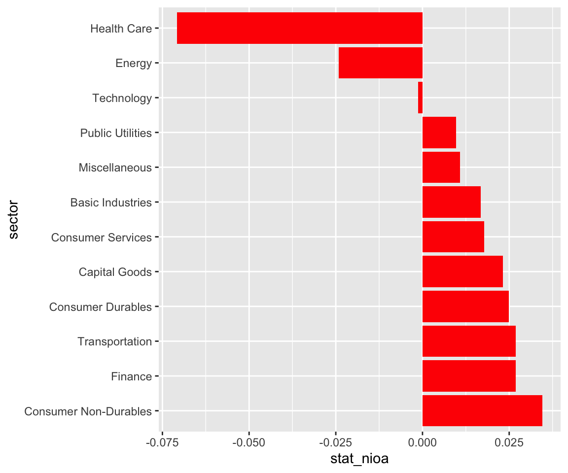
Whoa. This is not looking too good for the health sector. Let’s take a quick look at the distribution.
ret <- prepare_by_group_violin_graph(r3win, by_var = "sector", var = "nioa",
                                     order_by_mean = TRUE)
ret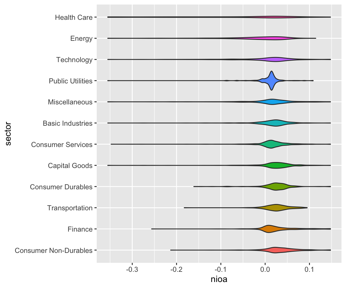
You can see that there is a relatively large mass of loss making firms in the health sector. This is not too surprising given that many publicly-listed health firms are relatively small growth firms. Also, you can see the effect of regulated profits in the public utilities sector.
Time Trends
Additional visuals are available for exploring time trends. prepare_trend_graph() can be used for comparing variables…
graph <- prepare_trend_graph(r3win[c("period", "nioa", "cfoa", "accoa")], "period")
graph$plot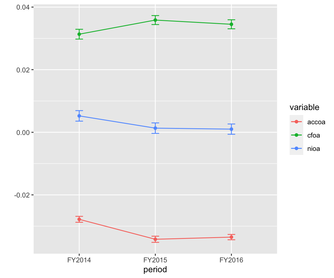
… and for eyeballing the distributional properties of a single variable over time you have prepare_quantile_trend_graph().
graph <- prepare_quantile_trend_graph(r3win[c("period", "return")], "period", c(0.05, 0.25, 0.5, 0.75, 0.95))
graph$plot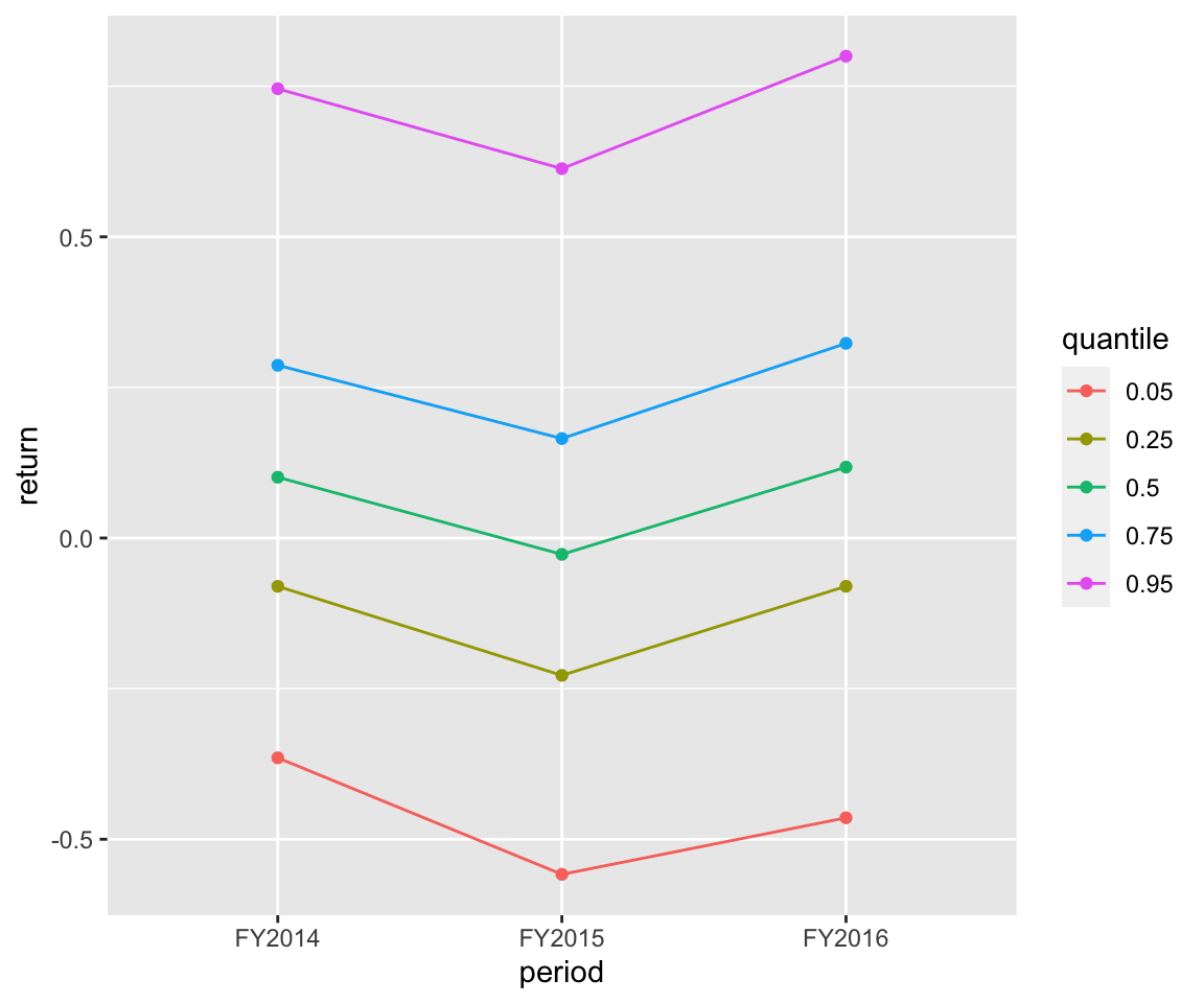
Nothing special going on here (not really surprising, given the short time span that the sample covers).
Correlation Analysis
I am sure that you won’t care but I am a big fan of correlation tables. prepare_correlation_table() prepares a table reporting Pearson correlations above and Spearman correlations below the diagonal.
t<- prepare_correlation_table(r3win, bold = 0.01, format="html")
t$kable_ret %>%
kable_styling("condensed", full_width = F, position = "center")| A | B | C | D | E | |
|---|---|---|---|---|---|
| A: toas | 0.10 | 0.07 | 0.08 | -0.00 | |
| B: nioa | 0.17 | 0.80 | 0.49 | 0.15 | |
| C: cfoa | 0.10 | 0.66 | -0.09 | 0.12 | |
| D: accoa | 0.20 | 0.38 | -0.30 | 0.07 | |
| E: return | 0.04 | 0.20 | 0.14 | 0.08 | |
| This table reports Pearson correlations above and Spearman correlations below the diagonal. The number of observations ranges from 6002 to 6643. Correlations with significance levels below 1% appear in bold print. |
In fact, I like correlations so much that especially for samples containing many variables I use prepare_correlation_graph() to display a graphic variant based on the corrplot package. See for yourself.
ret <- prepare_correlation_graph(r3win)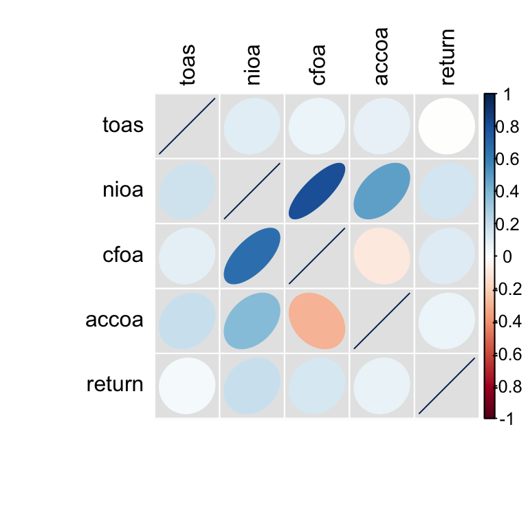
Scatter Plots
prepare_scatter_plot() produces the mother of all plots, the scatter plot. Here we take a look at the association of net income and stock returns.
prepare_scatter_plot(r3win, x="nioa", y="return", color="sector", size="toas", loess = 1)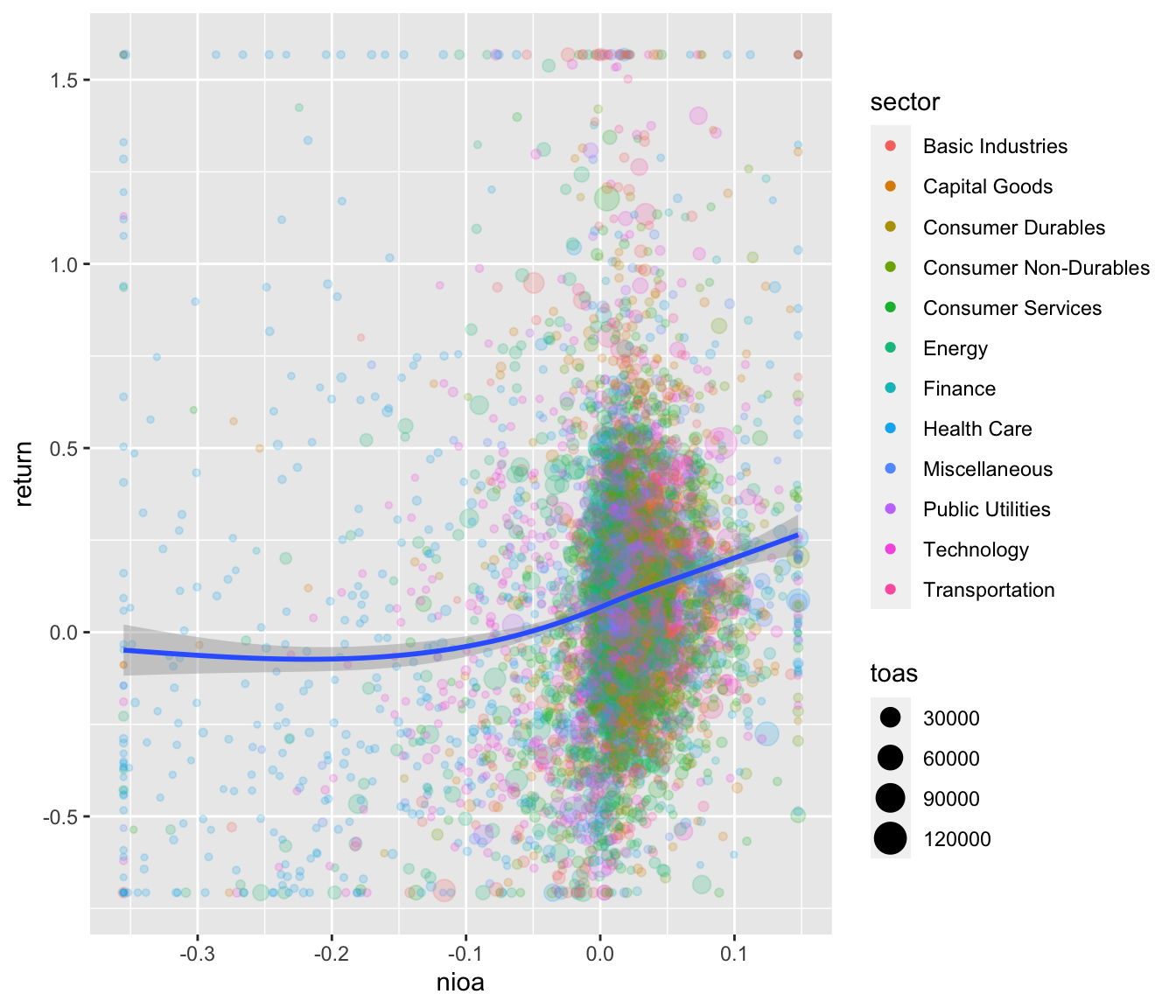
They are mildly positively associated indicating that more profitable firms also tend to have higher stock returns. Do you see the structural break around nioa == 0? This indicates that firms and/or the stock market treats losses differently than gains. Researchers in the area of accounting tend to find that interesting.
Regression Tables
Finally, if you happen to be a fan of starred numbers, you can also quickly produce regression tables by using the function prepare_regression_table() that calls lfe::felm() for OLS and glm() for binary logit models. The tables are then constructed by calling stargazer::stargazer(), allowing for plain text, html and latex output.
You can construct tables by mixing different models…
dvs <- c("return", "return", "return", "return", "return", "return")
idvs <- list(c("nioa"),
             c("cfoa"),
             c("accoa"),
             c("cfoa", "accoa"),
             c("nioa", "accoa"),
             c("nioa", "accoa"))
feffects <- list("period", "period", "period",
                 c("period", "coid"), c("period", "coid"), c("period", "coid"))
clusters <- list("", "", "", c("coid"), c("coid"), c("period", "coid"))
t <- prepare_regression_table(r3win, dvs, idvs, feffects, clusters)
htmltools::HTML(t$table)| Dependent variable: | ||||||
| return | return | return | return | return | return | |
| (1) | (2) | (3) | (4) | (5) | (6) | |
| nioa | 0.772*** | 1.794*** | 1.794** | |||
| (0.064) | (0.305) | (0.406) | ||||
| cfoa | 0.705*** | 1.582*** | ||||
| (0.073) | (0.326) | |||||
| accoa | 0.534*** | 0.876*** | -0.890*** | -0.890 | ||
| (0.116) | (0.303) | (0.314) | (0.440) | |||
| Estimator | ols | ols | ols | ols | ols | ols |
| Fixed effects | period | period | period | period, coid | period, coid | period, coid |
| Std. errors clustered | No | No | No | coid | coid | period, coid |
| Observations | 6,002 | 6,002 | 6,002 | 6,002 | 6,002 | 6,002 |
| R2 | 0.054 | 0.047 | 0.035 | 0.341 | 0.344 | 0.344 |
| Adjusted R2 | 0.054 | 0.046 | 0.035 | -0.044 | -0.039 | -0.039 |
| Note: | *p<0.1; **p<0.05; ***p<0.01 | |||||
… or by applying one model on different sub-samples.
t <- prepare_regression_table(r3win, "return", c("nioa", "accoa"), byvar="period")
htmltools::HTML(t$table)| Dependent variable: | ||||
| return | ||||
| Full Sample | FY2014 | FY2015 | FY2016 | |
| (1) | (2) | (3) | (4) | |
| nioa | 0.801*** | 0.234* | 0.607*** | 1.375*** |
| (0.074) | (0.139) | (0.123) | (0.119) | |
| accoa | -0.067 | 0.014 | 0.638*** | -1.224*** |
| (0.132) | (0.240) | (0.205) | (0.233) | |
| Constant | 0.082*** | 0.130*** | 0.014 | 0.096*** |
| (0.006) | (0.011) | (0.011) | (0.011) | |
| Estimator | ols | ols | ols | ols |
| Fixed effects | None | None | None | None |
| Std. errors clustered | No | No | No | No |
| Observations | 6,002 | 1,817 | 2,033 | 2,152 |
| R2 | 0.023 | 0.002 | 0.033 | 0.058 |
| Adjusted R2 | 0.023 | 0.001 | 0.032 | 0.057 |
| Note: | *p<0.1; **p<0.05; ***p<0.01 | |||
Conclusion
This is all there is (currently). All these functions are rather simple wrappers around established R functions. They can easily be modified to fit your needs and taste. Take look at the github repository of the ExPanDaR package for the code and do not hesitate to touch base for feedback. Enjoy!

