
reghdfe and R: The Joys of Standard Error Correction
I am an applied economist and economists love Stata. Every time I work with somebody who uses Stata on panel models with fixed effects and clustered standard errors I am mildly confused by Stata’s ‘reghdfe’ function producing standard errors that differ from common R approaches like the {sandwich}, {plm} and {lfe} packages.
Also, I recently had to update my {ExPanDaR} package to use the {plm} package as my favorite fixed effect package {lfe} was temporarily unavailable on CRAN. After doing that I decided that I finally want to understand what causes standard errors to differ across these packages. It was an interesting exercise and I summarize it here. Before reading further, here is the DISCLAIMER: I learned most of the below from trial and error over the last days and cannot guarantee correctness. I am very thankful for any feedback and corrections.
Act 1: Yet another R package
When starting to dive into the topic I discovered the {fixest} package. I was not aware of this package but it is now my favorite package for fixed effect models. It has a very smart user interface. What I like most about it that it separates standard error calculation from model estimation. That means that changing the standard errors is quick. Also, it comes with many options that make it easy to compare standard errors to those that other packages generate.
The vignette of the package about standard errors is extremely useful to understand the underlying issues. It also contains valuable pointers to the relevant literature on the topic. For me this is a must read if you want to dive deeper and don’t know where to start.
Act 2: Setting the Stage
To compare the various approaches, I use the Petersen dataset. While this also comes with the {sandwich} package I decided to download the version from Mitchell Petersen’s website. Also, I needed a way to call Stata from within R so that I can obtain the standard errors from ‘reghdfe’ and the ‘cluster2’ macro. Here we go:
library(dplyr)
library(tidyr)
library(broom)
library(foreign)
library(readr)
library(ggplot2)

# https://www.kellogg.northwestern.edu/faculty/petersen/htm/papers/se/test_data.htm
# for data and Standard Errors. Also see
# https://www.kellogg.northwestern.edu/faculty/petersen/htm/papers/se/se_programming.htm
# and https://sites.google.com/site/waynelinchang/r-code
# for some additional coding advice

df_petersen <- read.dta(
  "https://www.kellogg.northwestern.edu/faculty/petersen/htm/papers/se/test_data.dta"
)

# These are the coefficient as stated on the webpage
se_petersen <- list(
  ols = 0.0286,
  white = 0.0284,
  clustered_firm = 0.0506,
  clustered_year = 0.0334,
  clustered_fyear = 0.0536
)

# This my small function to call Stata from within R. You would need to
# adjust it if you want to use it in non-unix environments (Windows)
stata_path <- "/Applications/Stata/StataSE.app/Contents/MacOS/StataSE"
stata_path <- "/Applications/Stata/StataSE.app/Contents/MacOS/stata-se"

do_stata_file <- function(do_file, spath = stata_path, log = FALSE) {
  if(.Platform$OS.type != "unix") stop(
    "This only works on unix type OSes (inlcuding MacOS)."
  )
  if (log) system(paste(spath, "-b", do_file))
  else system(sprintf("%s < %s > /dev/null 2>&1", spath, do_file))
}

do_stata_file("../../static/code/petersen_clustered.do")

se_stata <- read_tsv("stata_se.tsv", col_types = cols())
The code calls a small Stata Do-file. Here is the file.
webuse set https://www.kellogg.northwestern.edu/faculty/petersen/htm/papers/se/
webuse test_data.dta, clear

file open tsv using "stata_se.tsv", write replace
set more off

* Plain OLS
reg y x

file write tsv "type" _tab "value" _n  "ols" _tab (_se[x]) _n

* OLS with robust SE
reg y x, robust
file write tsv "robust" _tab (_se[x]) _n

* OLS with SE clustered by firm
* The following needs  ssc install reghdfe
reghdfe y x, noabsorb cluster(firmid)
* equal to reg y x, vce(cluster firmid)
file write tsv "clustered_firm" _tab (_se[x]) _n

* OLS with SE clustered by year
reghdfe y x, noabsorb cluster(year)
* equal to reg y x, vce(cluster year)
file write tsv "clustered_year" _tab (_se[x]) _n

* The following needs the Petersen cluster2.ado file in your personal
* ado folder
cluster2 y x, fcluster(firmid)  tcluster(year)
file write tsv "clustered_fyear_petersen" _tab (_se[x]) _n

* OLS with SE clustered by firm and year
reghdfe y x, noabsorb cluster(firmid year)
file write tsv "clustered_fyear_reghdfe" _tab (_se[x]) _n

* Firm fixed effects with firm clusters
reghdfe y x, absorb(firmid) cluster(firmid)
file write tsv "fe_firm" _tab (_se[x]) _n

* Year fixed effects with year clusters
reghdfe y x, absorb(year) cluster(year)
file write tsv "fe_year" _tab (_se[x]) _n

* Two-way fixed effects with two-way clusters
reghdfe y x, absorb(firmid year) cluster(firmid year)
file write tsv "fe_fyear" _tab (_se[x]) _n
file close tsv
After running that file we cam compare the Stata results with the results from Petersen’s web page:
kable(se_stata) %>% kable_styling() | type | value |
|---|---|
| ols | 0.0285833 |
| robust | 0.0283952 |
| clustered_firm | 0.0505957 |
| clustered_year | 0.0333889 |
| clustered_fyear_petersen | 0.0535580 |
| clustered_fyear_reghdfe | 0.0552974 |
| fe_firm | 0.0301450 |
| fe_year | 0.0333835 |
| fe_fyear | 0.0296793 |
You see that (a) the standard errors generated by Stata are identical to the standard errors that are listed on Mitchell Petersen’s web page and (b) that ‘reghdfe’ calculates standard errors that differ from the standard errors generated by the original Petersen’s code. Here we go: The joy of standard error calculation for models with fixed effect and two-way clustered standard errors.
Act 3: Comparing Stata Standard Errors with {fixest} Standard Errors
The {fixest} package uses defaults that are identical to those of ‘reghdfe’ so it should be easy to get identical standard errors. Here is the code:
library(fixest)

mod_fixest_ols <- feols(y ~ x, data = df_petersen)
mod_fixest_fe_year <- feols(y ~ x | year, data = df_petersen)
mod_fixest_fe_firm <- feols(y ~ x | firmid, data = df_petersen)
mod_fixest_fe_fyear <- feols(y ~ x | year + firmid, data = df_petersen)

se_r_fixest <- list(
  ols = tidy(mod_fixest_ols)$std.error[2],
  robust = tidy(mod_fixest_ols, se = "hetero")$std.error[2],
  clustered_firm = tidy(mod_fixest_ols, cluster = "firmid")$std.error[2],
  clustered_year = tidy(mod_fixest_ols, cluster = "year")$std.error[2],
  clustered_fyear_petersen = tidy(
    mod_fixest_ols, cluster = c("firmid", "year"),
    dof = dof(cluster.df = "conv")
  )$std.error[2],
  clustered_fyear_reghdfe = tidy(
    mod_fixest_ols, cluster = c("firmid", "year")
  )$std.error[2],
  fe_firm = tidy(mod_fixest_fe_firm, cluster = "firmid")$std.error,
  fe_year = tidy(mod_fixest_fe_year, cluster = "year")$std.error,
  fe_fyear = tidy(mod_fixest_fe_fyear, cluster = c("firmid", "year"))$std.error
)
I use the very useful {broom} package to extract the standard errors. You see the design of the {fixest} package at work here: I only estimate the plain OLS version of the model once and then calculate different standard errors by repeating calls to tidy(). You could do the same with summary() calls.
Now the standard errors do look very similar. Are they identical, given the range of numerical precision?
se_fixest <- tibble(
  type = names(se_r_fixest),
  se_fixest = unname(unlist(se_r_fixest))
)

df <- se_stata %>% rename(se_stata = value) %>%
  left_join(se_fixest, by = "type") %>%
  mutate(equal = abs(se_stata - se_fixest) < 1e-7)

kable(df) %>% kable_styling()| type | se_stata | se_fixest | equal |
|---|---|---|---|
| ols | 0.0285833 | 0.0285833 | TRUE |
| robust | 0.0283952 | 0.0283952 | TRUE |
| clustered_firm | 0.0505957 | 0.0505957 | TRUE |
| clustered_year | 0.0333889 | 0.0333889 | TRUE |
| clustered_fyear_petersen | 0.0535580 | 0.0535580 | TRUE |
| clustered_fyear_reghdfe | 0.0552974 | 0.0552974 | TRUE |
| fe_firm | 0.0301450 | 0.0301450 | TRUE |
| fe_year | 0.0333835 | 0.0333835 | TRUE |
| fe_fyear | 0.0296793 | 0.0296790 | FALSE |
Hmpf. The standard errors for the two-way fixed effect model with two-way clustering are very close but not identical. This looks as if it could be a numerical precision case, though. Is it?
Act 4: The Rabbit Hole
I wanted to be sure. So I ran some simulations with varying samples:
set.seed(4242)

get_reghdfe_se <- function(df) {
  csv_file <- tempfile(fileext = ".csv")
  write_csv(df, file = csv_file)
  do_file <- tempfile(fileext = ".do")
  cat(sprintf(
    '
    import delimited %s, numericc(_all)
    reghdfe y x, absorb(firmid year) vce(cluster firmid year)
    file open ofile using "stata_regdhfe_coefs.txt", write replace
    file write ofile (_b[x]) _n (_se[x]) _n
    file close ofile
  ', csv_file
  ),
  file = do_file)
  do_stata_file(do_file)
  as.numeric(read_lines("stata_regdhfe_coefs.txt"))
}

get_fixest_se <- function(df, test_opt = FALSE) {
  mod_fixest_fe_fyear <- feols(
    y ~ x | firmid + year, data = df, fixef.rm = "both"
  )
  tidy(mod_fixest_fe_fyear, cluster = c("firmid", "year")) %>%
    select(estimate, std.error) %>%
    unlist(use.names=FALSE)
}

sim_df <- function(
  firms = 500, years = 10, effect = 1, pct_singleton = 0, pct_missing = 0
) {
  time_error_variance <- runif(years, 0.5, 1.5)
  firm_error_variance <- runif(firms, 0.5, 1.5)
  firm_is_singleton <- sample(
    c(rep(TRUE, as.integer(pct_singleton * firms)),
      rep(FALSE, firms - as.integer(pct_singleton * firms)))
  )
  sim_firm_data <- function(firmid) {
    if(firm_is_singleton[firmid]) {
      start_yr <- end_yr <- sample(1:years, 1)
    } else {
      start_yr <- 1
      end_yr <- years
    }
    n <- end_yr - start_yr + 1
    tibble(
      firmid = firmid,
      year = start_yr:end_yr,
      x = rnorm(n),
      y = effect*x +
        rnorm(rep(1, n), 0, time_error_variance[year]) +
        rnorm(n, 0, firm_error_variance[firmid]) +
        rnorm(n)
    )
  }

  df <- do.call(rbind, lapply(1:firms, sim_firm_data))
  obs_is_na <- sample(
    c(rep(TRUE, as.integer(pct_missing * nrow(df))),
      rep(FALSE, (firms - sum(firm_is_singleton))*years -
            as.integer(pct_missing * nrow(df))))
  )
  df$x[!firm_is_singleton[df$firmid]] <- ifelse(
    obs_is_na, NA, df$x[!firm_is_singleton[df$firmid]]
  )

  df$firmid <- as.factor(df$firmid)
  df$year <- as.factor(df$year)
  df
}


get_coefs <- function(
  firms = 500, years = 10, pct_singleton = 0, pct_missing = 0
) {
  message(sprintf(paste(
    "Estimating models on data for %d firms and %d years",
    "with %.2f%% singletons and %.2f%% missings"),
    firms, years, 100 * pct_singleton, 100 * pct_missing
  ))
  df <- sim_df(
    firms = firms, years = years,
    pct_singleton = pct_singleton, pct_missing = pct_missing
  )
  reghdfe <-  get_reghdfe_se(df)
  fixest <- get_fixest_se(df)
  tibble(
    firms = firms,
    years = years,
    pct_singleton = pct_singleton,
    pct_missing = pct_missing,
    reghdfe_b = reghdfe[1],
    reghdfe_se = reghdfe[2],
    fixest_b = fixest[1],
    fixest_se = fixest[2]
  )
}

df <- expand.grid(
  firms = c(10, 50, 100),
  years = 10,
  pct_singleton = seq(0, 0.3, 0.1),
  pct_missing = seq(0, 0.3, 0.1)
)

coefs <- do.call(
  rbind, lapply(1:nrow(df), function(x)
    get_coefs(df[x, 1], df[x, 2], df[x, 3], df[x, 4])
  )
) %>% mutate(
  n = as.integer((1 - pct_missing)*(1 - pct_singleton)*firms*years),
  diff = reghdfe_se - fixest_se
)

p_base <- ggplot(coefs, aes(y = diff)) +
  theme_classic()

p_base + geom_point(aes(x = n)) 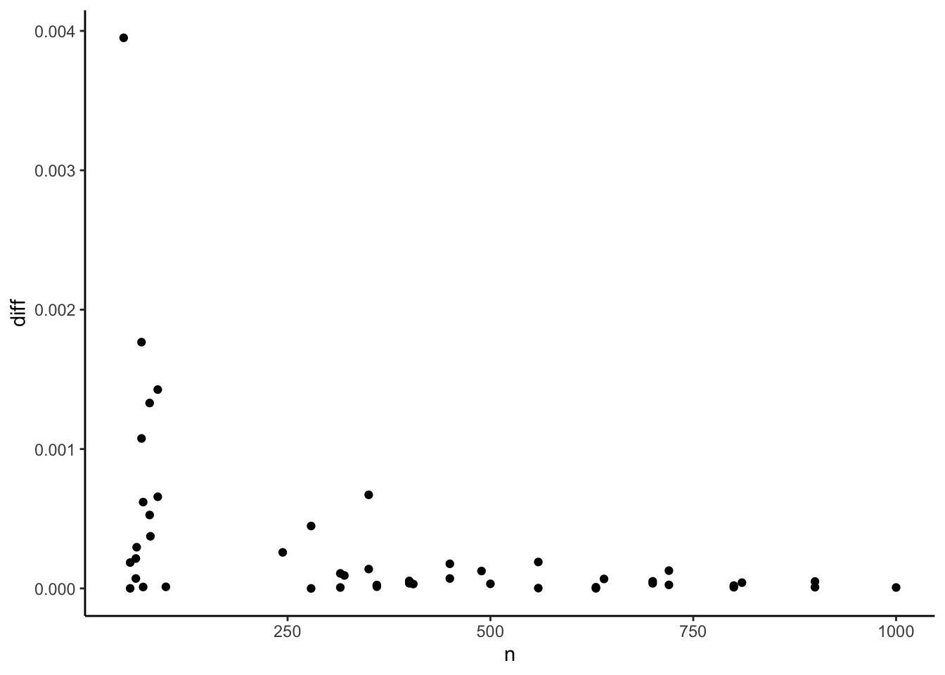
This does not look like a numerical precision issue. The differences are too large. The pattern seems to indicate that they become larger with smaller samples. This observation led me to spend some time digging through the degree of freedom correction procedures that ‘reghdfe’ and {fixest} use but no avail. In the end, I noticed an odd behavior in ‘reghdfe’: Since some time ago, it reports a constant coefficient by default even when fixed effects are present in the model. Why it does is beyond me, given that this constant cannot be interpreted in a meaningful way without diving into the internals of the fixed effect structure. An (unintended?) side effect of this is that ‘reghdfe’ has now to calculate a standard error for this meaningless constant. Sometimes this causes the Variance/Covariance matrix to become non-positive semi-definite and thus the application of the Cameron, Gelbach & Miller (2011, p. 241 f.) fix. This also affects the standard error of the independent variable marginally and causes the difference. At least this is my hunch after spending some time in this rabbit hole. Luckily, ‘reghdfe’ offers an undocumented ‘noconstant’ option. Let’s see whether this changes things:
get_reghdfe_se <- function(df) {
  csv_file <- tempfile(fileext = ".csv")
  write_csv(df, file = csv_file)
  do_file <- tempfile(fileext = ".do")
  cat(sprintf(
    '
    import delimited %s, numericc(_all)
    reghdfe y x, absorb(firmid year) vce(cluster firmid year) noconstant
    file open ofile using "stata_regdhfe_coefs.txt", write replace
    file write ofile (_b[x]) _n (_se[x]) _n
    file close ofile
  ', csv_file
  ),
  file = do_file)
  do_stata_file(do_file)
  as.numeric(read_lines("stata_regdhfe_coefs.txt"))
}

df <- expand.grid(
  firms = c(10, 50, 100),
  years = 10,
  pct_singleton = seq(0, 0.3, 0.1),
  pct_missing = seq(0, 0.3, 0.1)
)

coefs_new <- do.call(
  rbind, lapply(1:nrow(df), function(x)
    get_coefs(df[x, 1], df[x, 2], df[x, 3], df[x, 4])
  )
) %>% mutate(
  n = as.integer((1 - pct_missing)*(1 - pct_singleton)*firms*years),
  diff = reghdfe_se - fixest_se
)

options(digits = 7)

p_base <- ggplot(coefs_new, aes(y = diff)) +
  theme_classic()

p_base + geom_point(aes(x = n)) 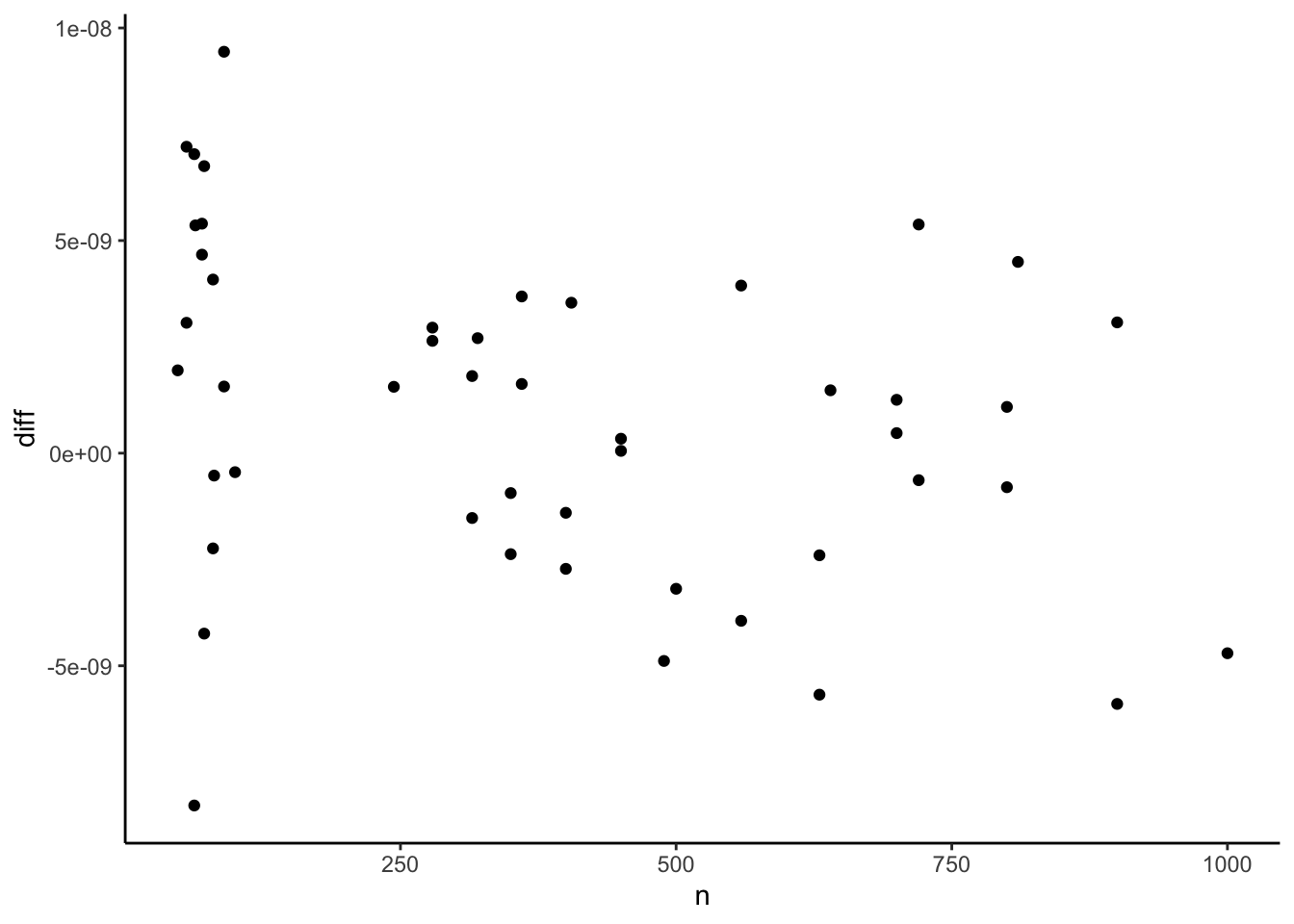
Yupp, it does. The differences are now all within numerical precision range. Great. By the way. I will file an issue with the ‘reghdfe’ maintainer about this. While this is to some extent the unavoidable cost for reporting a constant and its standard error maybe it would be nice to make this side effect more prominent.1
Act 5: What About Other Packages?
Now that we have established that {fixest} is capable to prepare standard errors that are identical to ‘reghdfe’ it is relatively straight-forward to compare the standard errors of the other packages. Let’s start with my long-time favorite {lfe}. As can be understood by reading this super informative Github issue {lfe} used to have a small sample correction that differed from the one of ‘reghdfe’ but has now an explicit option to make it “‘reghdfe’ compliant”.
library(lfe)

mod_felm_ols <- felm(y ~ x, data=df_petersen)
mod_felm_firm <- felm(y ~ x | 0 | 0 | firmid, data=df_petersen)
mod_felm_year <- felm(y ~ x | 0 | 0 | year, data=df_petersen)
mod_felm_fyear_petersen <- felm(y ~ x | 0 | 0 | firmid + year, data=df_petersen)
mod_felm_fyear_reghdfe <- felm(
  y ~ x | 0 | 0 | firmid + year, data=df_petersen, cmethod='reghdfe'
)
mod_felm_fe_firm <- felm(
  y ~ x | firmid | 0 | firmid, data=df_petersen, cmethod='reghdfe'
)
mod_felm_fe_year <- felm(
  y ~ x | year | 0 | year, data=df_petersen, cmethod='reghdfe'
)
mod_felm_fe_fyear <- felm(
  y ~ x | year + firmid | 0 | year + firmid, data=df_petersen, cmethod='reghdfe'
)

se_r_lfe <- list(
  ols = tidy(mod_felm_ols)$std.error[2],
  robust = tidy(mod_felm_ols, se.type = "robust")$std.error[2],
  clustered_firm = tidy(mod_felm_firm)$std.error[2],
  clustered_year = tidy(mod_felm_year)$std.error[2],
  clustered_fyear_petersen = tidy(mod_felm_fyear_petersen)$std.error[2],
  clustered_fyear_reghdfe = tidy(mod_felm_fyear_reghdfe)$std.error[2],
  fe_firm = tidy(mod_felm_fe_firm)$std.error,
  fe_year = tidy(mod_felm_fe_year)$std.error,
  fe_fyear = tidy(mod_felm_fe_fyear)$std.error
)

se_lfe <- tibble(
  type = names(se_r_lfe),
  se_lfe = unname(unlist(se_r_lfe))
)

df <- se_fixest %>%
  left_join(se_lfe, by = "type") %>%
  mutate(equal = abs(se_fixest - se_lfe) < 1e-7)

kable(df) %>% kable_styling()| type | se_fixest | se_lfe | equal |
|---|---|---|---|
| ols | 0.0285833 | 0.0285833 | TRUE |
| robust | 0.0283952 | 0.0283952 | TRUE |
| clustered_firm | 0.0505957 | 0.0505957 | TRUE |
| clustered_year | 0.0333889 | 0.0333889 | TRUE |
| clustered_fyear_petersen | 0.0535580 | 0.0535580 | TRUE |
| clustered_fyear_reghdfe | 0.0552974 | 0.0552974 | TRUE |
| fe_firm | 0.0301450 | 0.0301450 | TRUE |
| fe_year | 0.0333835 | 0.0333835 | TRUE |
| fe_fyear | 0.0296790 | 0.0296790 | TRUE |
This looks good. But keep in mind that, different from {fixest} with the ‘fixef.rm’ option and ‘reghdfe’, {lfe} does not automatically delete singleton observations (observations that are uniquely identified by a fixed effect) before estimating the model. While the Petersen data set is perfectly balanced and thus has no singletons, singletons will regularly exist in real-life research settings.
Next, we turn to the good old {sandwich} package. Together with {lmtest}, it allows the flexible calculation of various robust standard errors. It does not, however, use the exact same degrees of freedom correction that {fixest} and ‘reghdfe’ use. First, it does not address the problem of nested fixed effects, meaning fixed effects that only vary within clusters. Second, it uses the weighted cluster correction while ‘reghdfe’/{fixest} use the minimum cluster correction.2
To understand this, I whipped up a hacky function that manually calculates the degree of freedom correction based on the clusters and fixed effects. This is largely untested and will work only on regular fixed effect/cluster structures but helped me to understand the issue better. Here it is:
dofcorr <- function(
  N, kvars, cmat, femat, fixef.K = "nested", cluster.adj = TRUE
) {
  # N:     Number of observations used in model estimation
  # kvars: Number of all normal variables in the model
  #        (without fixed effects but including the intercept)
  # cmat:  Matrix with N rows containing all clusters
  # femat: Matrix with N rows containing all fixed effects
  # Other arguments as in ?fixest::dof
  # NOT FOR PRODUCTION - Only for didactic purposes
  # Will not work on irregular fixed effects and clusters
  # See https://lrberge.github.io/fixest/articles/standard_errors.html
  # for guidance

  k <- switch(
    fixef.K,
    "none" = 0,
    "full" = sum(apply(femat, 2, function (x) {length(unique(x)) - 1})),
    "nested" = {
      sum(apply(femat, 2, function (fe) {
        fes <- unique(fe)
        min(unlist(apply(
          cmat, 2, function(cl) {
            sum(unlist(lapply(fes, function(fes)
              ifelse(length(unique(cl[fe == fes])) > 1, 1, 0)
            )))
          }
        )))
      }
      ))
    }
  ) + kvars
  ssc <- (N - 1)/(N - k)
  if (!cluster.adj) return(ssc)
  G <- min(apply(femat, 2, function (x) length(unique(x))))
  G/(G - 1) * ssc
}
With this, we can now adjust the {sandwich} VCOVs as long as the data is well behaved. For this we need to use its functions to calculate a clustered but unadjusted VCOV by setting type = "HC0" and cadjust = FALSE.
library(sandwich)
library(lmtest)

mod_ols <- lm(y ~ x, data = df_petersen)
mod_ols_fe_firm <- lm(y ~ x + as.factor(firmid), data = df_petersen)
mod_ols_fe_year <- lm(y ~ x + as.factor(year), data = df_petersen)
mod_ols_fe_fyear <- lm(
  y ~ x + as.factor(firmid) + as.factor(year), data = df_petersen
)

se_r_sandwich <- list(
  ols = tidy(mod_ols)$std.error[2],
  robust = coeftest(mod_ols, vcov = vcovHC(mod_ols, type = "HC1"))[2, 2],
  clustered_firm =  coeftest(
    mod_ols, vcov = vcovCL(mod_ols, cluster = ~ firmid)
  )[2, 2],
  clustered_year =  coeftest(
    mod_ols, vcov = vcovCL(mod_ols, cluster = ~ year)
  )[2, 2],
  clustered_fyear_petersen =  coeftest(
    mod_ols, vcov = vcovCL(mod_ols, cluster = ~ firmid + year)
  )[2, 2],
  clustered_fyear_reghdfe =  coeftest(
    mod_ols,
    vcov = vcovCL(mod_ols, cadjust = FALSE, cluster = ~ firmid + year)*(10/9)
  )[2, 2],
  fe_firm = coeftest(
    mod_ols_fe_firm,
    vcov = dofcorr(
      nrow(df_petersen), 2,
      df_petersen %>% select(firmid),
      df_petersen %>% select(firmid)
    ) * vcovCL(mod_ols_fe_firm, type = "HC0", cadjust = FALSE, cluster = ~ firmid)
  )[2, 2],
  fe_year = coeftest(
    mod_ols_fe_year,
    vcov = dofcorr(
      nrow(df_petersen), 2,
      df_petersen %>% select(year),
      df_petersen %>% select(year)
    ) * vcovCL(mod_ols_fe_year, type = "HC0", cadjust = FALSE, cluster = ~ year)
  )[2, 2],
  fe_fyear =  coeftest(
    mod_ols_fe_fyear,
    vcov =  dofcorr(
      nrow(df_petersen), 2,
      df_petersen %>% select(year, firmid),
      df_petersen %>% select(year, firmid)
    ) * vcovCL(
      mod_ols_fe_fyear, type = "HC0", cadjust = FALSE, cluster = ~ firmid + year
    )
  )[2, 2]
)

se_sandwich <- tibble(
  type = names(se_r_sandwich),
  se_sandwich = unname(unlist(se_r_sandwich))
)

df <- se_fixest %>%
  left_join(se_sandwich, by = "type") %>%
  mutate(equal = abs(se_fixest - se_sandwich) < 1e-7)

kable(df) %>% kable_styling()| type | se_fixest | se_sandwich | equal |
|---|---|---|---|
| ols | 0.0285833 | 0.0285833 | TRUE |
| robust | 0.0283952 | 0.0283952 | TRUE |
| clustered_firm | 0.0505957 | 0.0505957 | TRUE |
| clustered_year | 0.0333889 | 0.0333889 | TRUE |
| clustered_fyear_petersen | 0.0535580 | 0.0535580 | TRUE |
| clustered_fyear_reghdfe | 0.0552974 | 0.0552974 | TRUE |
| fe_firm | 0.0301450 | 0.0301450 | TRUE |
| fe_year | 0.0333835 | 0.0333835 | TRUE |
| fe_fyear | 0.0296790 | 0.0296790 | TRUE |
And, finally, for the sake of completeness, the same approach for {plm}
# See Millo (2017): https://www.jstatsoft.org/article/view/v082i03
# and https://blog.theleapjournal.org/2016/06/sophisticated-clustered-standard-errors.html
# "sss" gives the small sample correction that is being used by standard {lfe}
# and 'reghdfe' for unnested fixed effects and one way clustering.
# See Millo(2017): 22f.

library(plm)

mod_plm <- plm(
  y ~ x, index = c("firmid", "year"), model = "pooling", df_petersen
)
mod_plm_fe_firm <- plm(
  y ~ x, index = c("firmid", "year"), model = "within",
  effect = "individual", df_petersen
)
mod_plm_fe_year <- plm(
  y ~ x, index = c("firmid", "year"), model = "within",
  effect = "time", df_petersen
)
mod_plm_fe_fyear <- plm(
  y ~ x, index = c("firmid", "year"), model = "within",
  effect = "twoways", df_petersen
)

se_r_plm <- list(
  ols = tidy(mod_plm)$std.error[2],
  robust = coeftest(
    mod_plm, vcov = vcovHC(mod_plm, method = "white1", type = "HC1")
  )[2, 2],
  clustered_firm = coeftest(
    mod_plm, vcov = vcovHC(mod_plm, type = "sss", cluster = "group")
  )[2, 2],
  clustered_year = coeftest(
    mod_plm, vcov = vcovHC(mod_plm, type = "sss", cluster = "time")
  )[2, 2],
  clustered_fyear_petersen = coeftest(
    mod_plm, vcov = vcovDC(mod_plm, type = "sss")
  )[2, 2],
  clustered_fyear_reghdfe = coeftest(
    mod_plm,
    vcov = dofcorr(
      nrow(df_petersen), 2,
      df_petersen %>% select(firmid, year),
      df_petersen %>% select(firmid, year)
    ) * vcovDC(mod_plm, type = "HC0")
  )[2, 2],
  fe_firm = coeftest(
    mod_plm_fe_firm,
    vcov = dofcorr(
      nrow(df_petersen), 2,
      df_petersen %>% select(firmid),
      df_petersen %>% select(firmid)
    ) * vcovHC(mod_plm_fe_firm, type = "HC0", cluster = "group")
  )[2],
  fe_year = coeftest(
    mod_plm_fe_year,
    vcov = dofcorr(
      nrow(df_petersen), 2,
      df_petersen %>% select(year),
      df_petersen %>% select(year)
    ) * vcovHC(mod_plm_fe_year, type = "HC0", cluster = "time")
  )[2],
  fe_fyear = coeftest(
    mod_plm_fe_fyear,
    vcov = dofcorr(
      nrow(df_petersen), 2,
      df_petersen %>% select(firmid, year),
      df_petersen %>% select(firmid, year)
    ) * vcovDC(mod_plm_fe_fyear, type = "HC0")
  )[2]
)

se_plm <- tibble(
  type = names(se_r_plm),
  se_plm = unname(unlist(se_r_plm))
)

df <- se_fixest %>%
  left_join(se_plm, by = "type") %>%
  mutate(equal = abs(se_fixest - se_plm) < 1e-7)

kable(df) %>% kable_styling()| type | se_fixest | se_plm | equal |
|---|---|---|---|
| ols | 0.0285833 | 0.0285833 | TRUE |
| robust | 0.0283952 | 0.0283952 | TRUE |
| clustered_firm | 0.0505957 | 0.0505957 | TRUE |
| clustered_year | 0.0333889 | 0.0333889 | TRUE |
| clustered_fyear_petersen | 0.0535580 | 0.0535580 | TRUE |
| clustered_fyear_reghdfe | 0.0552974 | 0.0552974 | TRUE |
| fe_firm | 0.0301450 | 0.0301450 | TRUE |
| fe_year | 0.0333835 | 0.0333835 | TRUE |
| fe_fyear | 0.0296790 | 0.0296790 | TRUE |
The Curtain
This is it. Apologies for the longish post. The main takeaway is that you should use noconstant when using ‘reghdfe’ and {fixest} if you are interested in a fast and flexible implementation for fixed effect panel models that is capable to provide standard errors that comply wit the ones generated by ‘reghdfe’ in Stata. If you are an economist this will likely make your coauthors happy.
Based on my understanding, the above should hold as long as your have regular fixed effects and clusters. When you have multiple fixed effects that partly overlap, like for example employees that change from one firm to another (executive compensation literature, I am looking at you) then it remains to be seen whether ‘reghdfe’ and {fixest} still agree on standard errors. This is another rabbit hole for another day…
Enjoy!
Update: Here is the link to the issue. As you will see, Sergio Correia already reacted to it and provided a fix in the current development version of ‘reghdfe’. Whow, just whow!↩︎
I apologize for this imprecise gibberish. I again recommend the wonderful standard error vignette of the {fixest} package for further information.↩︎

