
Interactive panel EDA with 3 lines of code
Exploratory data analysis is important, everybody knows that. With R, it is also easy. Below you see three lines of code that allow you to interactively explore the Preston Curve, the prominent association of country level real income per capita with life expectancy.
install.packages("ExPanDaR")
library(ExPanDaR)
wb <- read.csv("https://joachim-gassen.github.io/data/wb_condensed.csv")
ExPanD(wb, cs_id = "country", ts_id = "year")
After running these three lines of code (OK, four if you have to install the ExPanDaR package first), a shiny window will open, allowing you to explore a country-year panel of World Bank data and looking something like this.
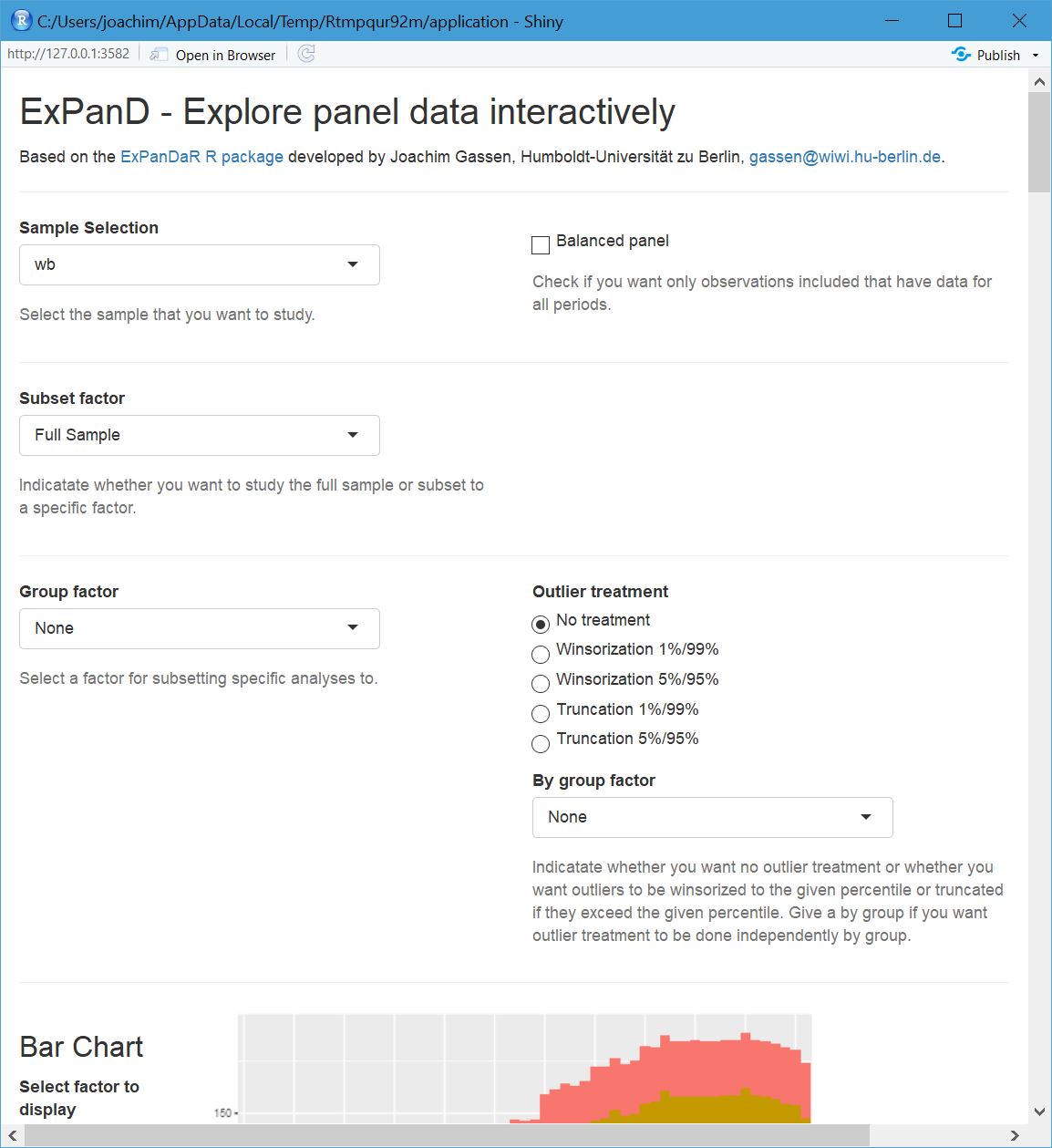
Screenshot of ExPanD window
If you do not have access to R, you can also access a version online. Explore away! When you scroll down, you will notice several issues:
- While
gdp_capitaandlifeexpectancyare available for all observations, a lot of the additional variables presented in the data set are only available for a subset of country-year observations. gdp_capitais heavily right skewed, meaning that many countries have low real income per capital while few countries have high levels. By looking at the extreme observations table, you can identify the usual suspects.- Not surprisingly, income is unevenly distributed across geographic regions. This also holds for life expectancy.
gdp_capitagrows over time and its distribution widens.lifeexpectancyalso grows but, luckily, its distribution does not widen over time.- The scatter plot of
gdp_capitaandlifeexpectancyconstitutes the Preston Curve, which was first documented in the seventies.
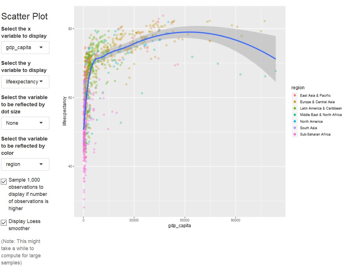
Preston Curve, as displayed by ExPanD
The regression results below the scatter plot document the positive association between real income per capita and life expectancy. But, when you look at the scatter plot carefully and hover over it with your mouse to identify observations, you will likely notice that countries seem to have their unique development patterns. This calls for the inclusion of country-level fixed effects in the regression.
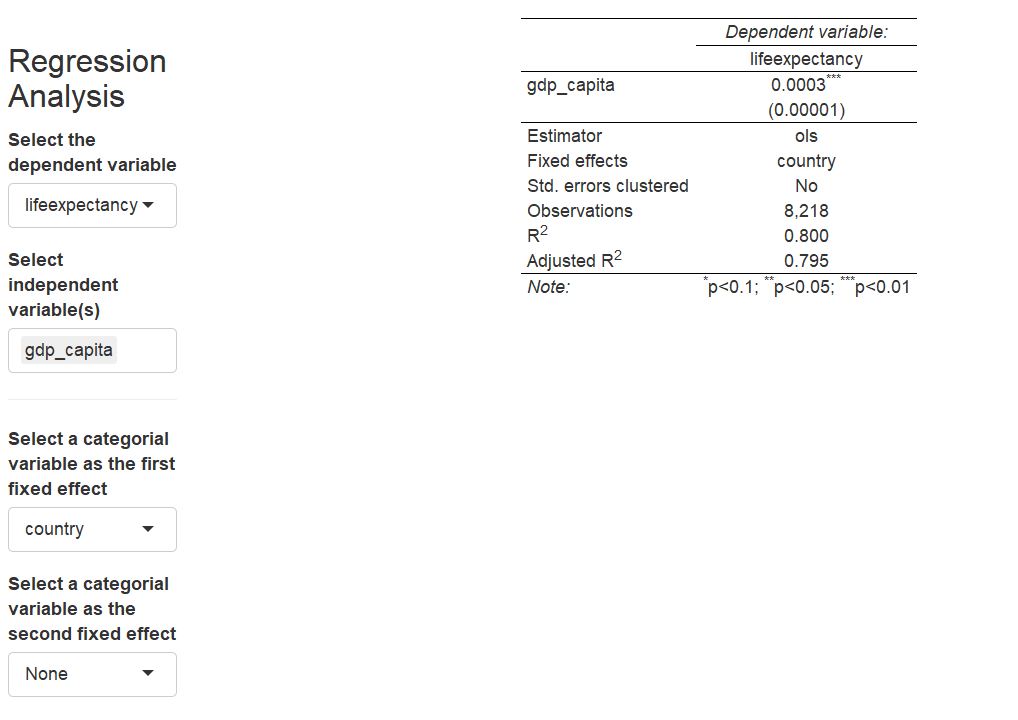
Regression results with country fixed effects
The association of real income with life expectancy is still there. But will it continue to hold when we allow life expectancy to follow a world-wide time trend? As medical advancements affect multiple countries more or less concurrently, this seems important to test. Let’s throw in some year fixed effects as well.
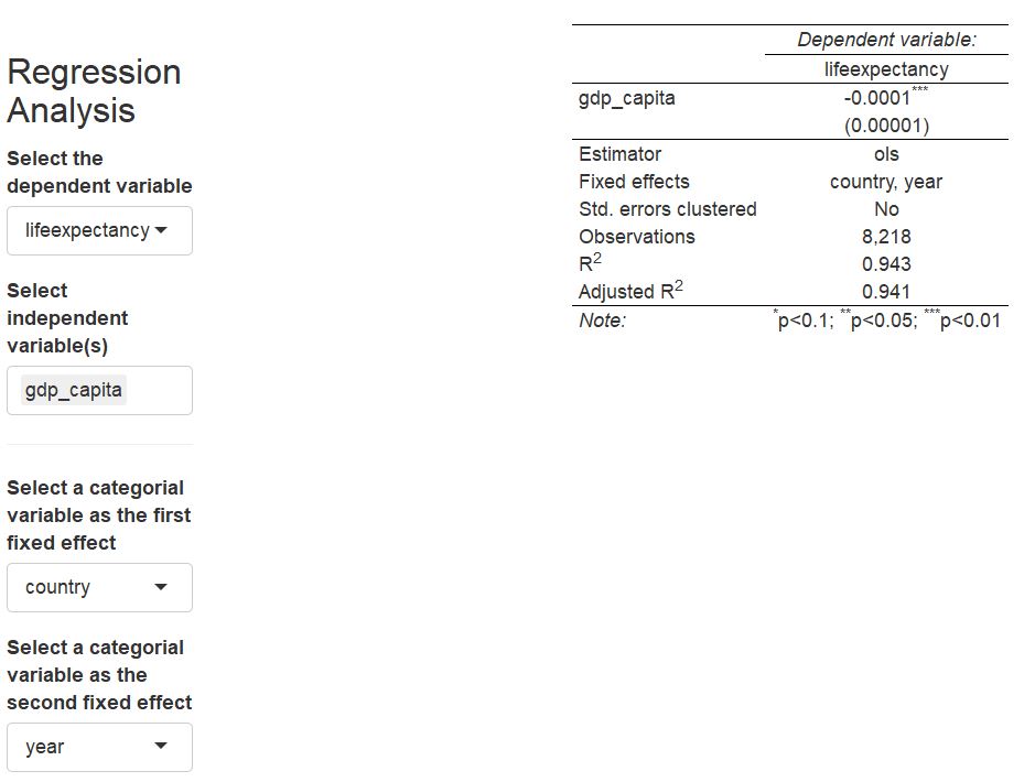
Regression results with country fixed effects
Uhuh. Now the association of real income per capita and life expectancy has turned negative! This indicates that higher real income per capita is associated with lower life expectancy after allowing for unobserved time and country heterogeneity. What do we learn from this exercise?
- Correlations do not imply causality.
- If we allow for the possibility that life expectancy changes over time because of global changes (like, e.g. medical discoveries, wars and conflicts) and that countries come from different starting grounds (e.g., because of their geographic location), then we cannot observe a robust association of real income per capita with life expectancy.
- Whether real income per capital has a causal effect on life expectancy cannot be assessed by a simplistic analysis like the one presented here and the Preston curve presenting the striking correlation can be easily miss-understood to indicate such a causation.
All this can be reached with three lines of R and some clicks. If you are interested to explore the Preston curve and the functions behind my ExPanDaR package in somewhat more detail, you can take a look at this kaggle kernel.
But hey, you might ask, I do not work with panel data, so why should I care? Well, while I developed the ExPanDaR package for panel data, you can squeeze it to use it on plain cross-sectional data. See below for a classic example:
library(ExPanDaR)
df <- mtcars
df$cs_id <- row.names(df)
df$ts_id <-1
ExPanD(df, cs_id ="cs_id", ts_id = "ts_id",
       components = c(trend_graph = FALSE, quantile_trend_graph = FALSE))
If you want to dive into the ExPanDaR package a little it more, here is its github page. It also contains the code to generate the data used here as well as the additional steps to generate the online version, including data definitions and a customized landing text for the ExPanD app.
Enjoy!

