Where the German Companies Are
Last week, the German NGO Open Knowledge Foundation Deutschland e.V. has made German Trade Resister data available via the project OffeneRegister.de, together with the British NGO opencorporates. While the data from German Trade Resister is publicly available in principle, retrieving the data is a case-by-case activity and is very cumbersome (try for yourself if you like). The data provided by OffeneRegister.de instead comes with an easy to navigate API, and, what is even more convenient, is available for bulk download (alternatively as a JSON or as a SQLite database file).
Having a research focus on corporate transparency, I could not resist the temptation to take a peak. I downloaded the SQLite database. Let’s access it with R.
library(DBI)
library(tidyverse)
library(ggmap)
library(rgdal)
library(rgeos)

# You will also need the packages R.utils, maproj, and RSQLite to run this code

tmp <- tempdir()
download.file("https://daten.offeneregister.de/openregister.db.gz",
              destfile = file.path(tmp, "openregister.db.gz"))
db <- R.utils::gunzip(file.path(tmp, "openregister.db.gz"))
con <- dbConnect(RSQLite::SQLite(), db)
While I have my reservations about using the individual data contained in the data base for data quality and privacy reasons, some aggregate analysis seems in order. As a proof of concept, I will try to visualize where German companies are located. Thus, I focus on the relation companies and try to extract some spatial variation.
sql <- "select id, current_status, retrieved_at, registered_address from company"
res <- dbSendQuery(con, sql)
company <- dbFetch(res)
dbClearResult(res)
dbDisconnect(con)
An inspection of the registered_address field shows that the data is relatively messy, but most non-empty cells contain five digit German post codes (Postleitzahlen, PLZ). I will focus on those.
company %>%
  filter(current_status == "currently registered",
         !is.na(registered_address)) %>%
  mutate(plz = str_extract(registered_address, "\\d{5}")) %>%
  filter(plz != "") %>%
  select(id, plz) -> company_plz
Time to ask our first question. What are the TOP 10 firm hosting PLZs?
companies_plz <- company_plz %>%
  group_by(plz) %>%
  summarise(companies = n()) %>%
  mutate(link = sprintf('<a href="https://www.suche-postleitzahl.org/plz-gebiet/%s" target="_blank">Link to map</a>', plz)) %>%
  arrange(-companies)

kable(head(companies_plz, 10), col.names = c("PLZ", "Registered companies", "Link to map"),
format.args = list(big.mark = ","))| PLZ | Registered companies | Link to map |
|---|---|---|
| 10117 | 5,858 | Link to map |
| 20457 | 4,678 | Link to map |
| 20354 | 4,677 | Link to map |
| 20095 | 3,574 | Link to map |
| 82031 | 3,334 | Link to map |
| 10719 | 2,854 | Link to map |
| 22767 | 2,593 | Link to map |
| 60325 | 2,313 | Link to map |
| 10707 | 2,309 | Link to map |
| 55129 | 2,223 | Link to map |
The top PLZ on the list looks oddly familiar… But the list is not really informative as PLZ vary in size. Let’s link this to some spatial information.
# Shape file is based on OSM data.
# Source: https://www.suche-postleitzahl.org/downloads

download.file("https://www.suche-postleitzahl.org/download_files/public/plz-gebiete.shp.zip",
              file.path(tmp, "shape5.zip"))
unzip(file.path(tmp, "shape5.zip"), exdir = tmp)
plz_polys <- readOGR(file.path(tmp, "plz-gebiete.shp"))

plz_polys$area_sqkm <- raster::area(plz_polys) / 1000000

# Population data is based on the 100m raster data from Zensus 2011.
# Downloaded from: https://www.suche-postleitzahl.org/downloads
# Further info:
# http://blog.suche-postleitzahl.org/post/132153774751/einwohnerzahl-auf-plz-gebiete-abbilden
# https://www.zensus2011.de/SharedDocs/Aktuelles/Ergebnisse/DemografischeGrunddaten.html?nn=3065474

pop <- read_csv("https://www.suche-postleitzahl.org/download_files/public/plz_einwohner.csv")

pop_by_plz <- data.frame(
  plz = plz_polys$plz,
  area_sqkm = plz_polys$area_sqkm,
  stringsAsFactors = FALSE
)

pop_by_plz %>%
  left_join(pop) %>%
  left_join(companies_plz) %>%
  replace_na(list(companies = 0)) %>%
  rename(population = einwohner) %>%
  mutate(comp_by_sqkm = companies/area_sqkm,
         comp_by_1000pop = 1000*companies/population) -> comp_by_plz
How many companies are included in this data?
tab <- comp_by_plz %>%
  mutate(pa = substr(plz, 1,1 )) %>%
  group_by(pa) %>%
  summarise(companies = sum(companies))
tab <- rbind(tab, data.frame(pa = "Total", companies = sum(tab$companies)))

kable(tab, col.names = c("Post Area", "Registered companies"),
format.args = list(big.mark = ","))| Post Area | Registered companies |
|---|---|
| 0 | 48,149 |
| 1 | 132,031 |
| 2 | 148,632 |
| 3 | 84,158 |
| 4 | 125,925 |
| 5 | 123,386 |
| 6 | 115,156 |
| 7 | 107,075 |
| 8 | 103,568 |
| 9 | 69,503 |
| Total | 1,057,583 |
Quite a few. Which reasonably populated PLZs are home to more firms than people?
kable(comp_by_plz %>%
        filter(population > 100,
               comp_by_1000pop > 1000) %>%
        arrange(-comp_by_1000pop),
      col.names = c("PLZ", "Area (km²)", "Population", "Registered companies", "Link to map",
                    "Companies by km²", "Companies by 1,000 inhabitants"),
format.args = list(big.mark = ",", digits = 2)) | PLZ | Area (km²) | Population | Registered companies | Link to map | Companies by km² | Companies by 1,000 inhabitants |
|---|---|---|---|---|---|---|
| 40212 | 0.43 | 543 | 1,390 | Link to map | 3,219 | 2,560 |
| 20354 | 1.30 | 2,273 | 4,677 | Link to map | 3,600 | 2,058 |
| 20457 | 14.50 | 2,566 | 4,678 | Link to map | 323 | 1,823 |
| 20095 | 0.76 | 3,172 | 3,574 | Link to map | 4,704 | 1,127 |
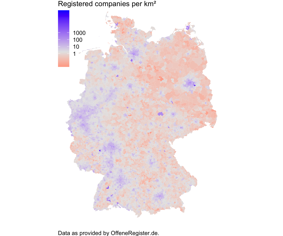
Interesting, Düsseldorf and Hamburg make the cut. Maps. We want to see maps. First: Registered companies by square kilometer.
# For visualization, values are log transformed. Set zero values to
# be 80 % of non-zero minimum to make them plottable.

min_1000pop <- 0.8 * min(comp_by_plz$comp_by_1000pop[comp_by_plz$comp_by_1000pop > 0], na.rm = TRUE)
min_sqkm <- 0.8 * min(comp_by_plz$comp_by_sqkm[comp_by_plz$comp_by_sqkm > 0], na.rm = TRUE)
log_safe <- comp_by_plz %>%
  mutate(comp_by_1000pop = replace(comp_by_1000pop,
                                   comp_by_1000pop == 0, min_1000pop),
         comp_by_sqkm = replace(comp_by_sqkm,
                                   comp_by_sqkm == 0, min_sqkm))

plz_map <-
  fortify(plz_polys, region = "plz") %>%
  left_join(log_safe, by = c("id" = "plz"))


ggplot(plz_map, aes(x = long, y = lat, group = group, fill = comp_by_sqkm)) +
  geom_polygon(colour = NA, lwd=0, aes(group = group)) +
  scale_fill_gradient2(name = "Registered companies per km²",
                       low = "red", mid = "gray90", high = "blue", trans = "log",
                       midpoint = log(median(log_safe$comp_by_sqkm, na.rm = TRUE)),
                       breaks = c(1, 10, 100, 1000)) +
  coord_map() +
  theme_void() +
  theme(legend.justification=c(0,1), legend.position=c(0,1), plot.caption = element_text(hjust = 0)) +
  labs(caption = "Data as provided by OffeneRegister.de.")
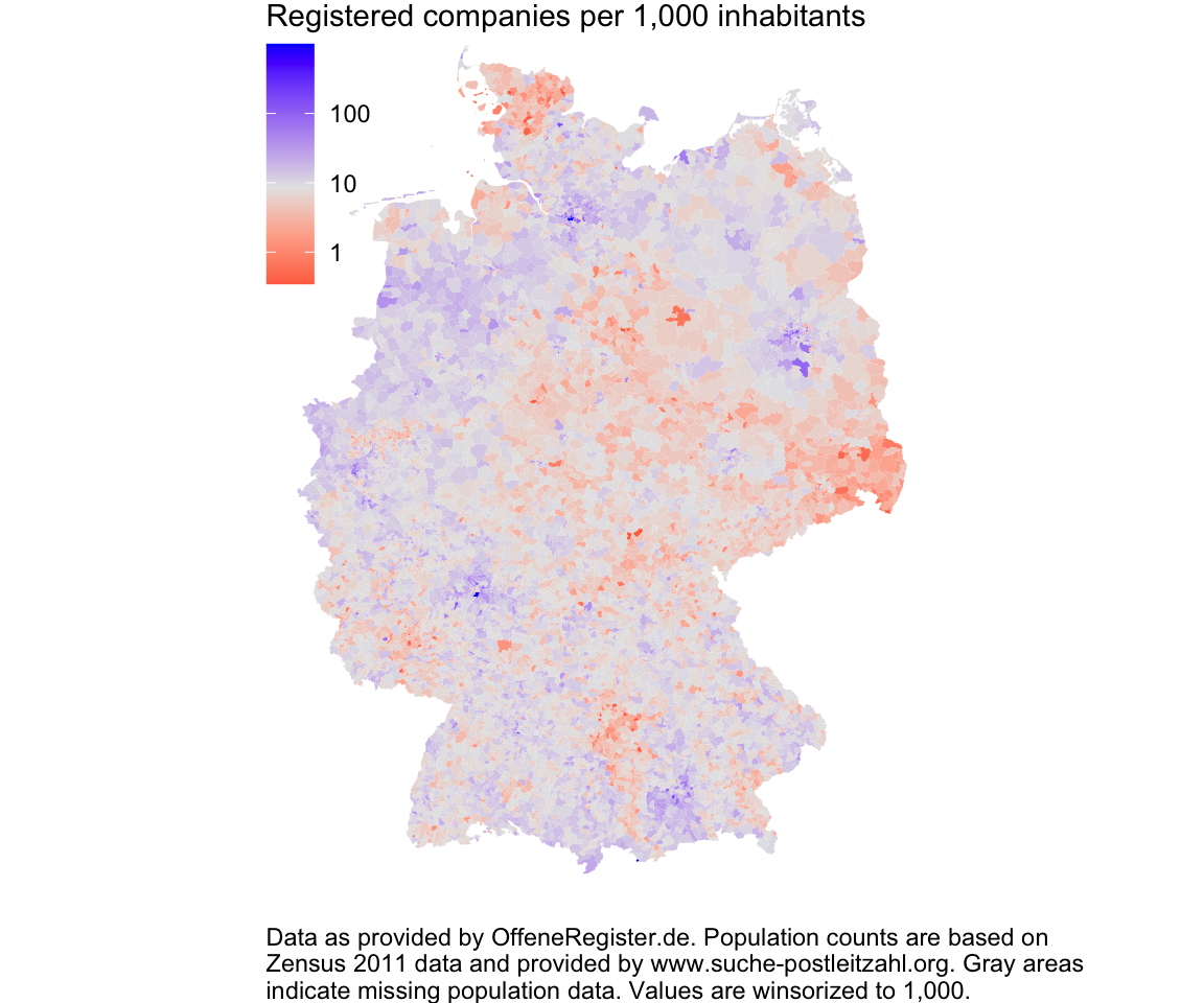
Nice but not really surprising. Some areas stand out (Ost-Westfalen Lippe and the Rhein valley) but in general companies are where people live (meaning: in cities). Do we get better insights when we plot registered companies relative to the population?
# As we have seen above, we have some few PLZs with rather extreme companies
# by population ratios. I set them to 1000 so that they do not mess up the scale

plz_map$comp_by_1000pop[plz_map$comp_by_1000pop > 1000] <- 1000

ggplot(plz_map, aes(x = long, y = lat, group = group, fill = comp_by_1000pop)) +
  geom_polygon(colour = NA, lwd=0, aes(group = group)) +
  scale_fill_gradient2(name = "Registered companies per 1,000 inhabitants",
                       low = "red", mid = "gray90", high = "blue", trans = "log",
                       midpoint = log(median(log_safe$comp_by_1000pop, na.rm = TRUE)),
                       breaks = c(1, 10, 100)) +
  coord_map() +
  theme_void() +
  theme(legend.justification=c(0,1), legend.position=c(0,1), plot.caption = element_text(hjust = 0)) +
  labs(caption = paste("Data as provided by OffeneRegister.de. Population counts are based on",
                       "Zensus 2011 data and provided by www.suche-postleitzahl.org. Gray areas",
                       "indicate missing population data. Values are winsorized to 1,000.", sep = "\n"))
Now this is interesting. You can see relatively strong regional patterns. Some cities are not as company heavy as others (compare Leipzig to Dresden and see the Ruhr area). Some rural areas show higher levels of corporate activity (North Brandenburg, Mecklenburg) while others have relatively low levels (North Schleswig-Holstein, Saxonia, Swabia in Bavaria).
A larger version of the plot above (with a base map for better orientation) can be downloaded here.
Summing up: The data provided by OffeneRegister.de, while being somewhat messy at the individual level, can be used to generate informative insights at the aggregate level. Let’s hope that the initiative helps to trigger a public debate about the right way to host public data.
