Taking Outlier Treatment to the Next Level
By Joachim Gassen (Humboldt University Berlin, TRR 266 “Accounting for Transparency”) and David Veenman (University of Amsterdam)
“To reduce the impact of outliers on our findings, we winsorize the dependent and independent variables at the top and bottom percentile.” If you do empirical archival research in accounting and/or corporate finance, we bet that you have read and written such a sentence many times throughout your career. We know that outliers exist and that we have to “deal” with them. As Mitton (RFS, 2021) shows, outlier treatment is among the most impactful design choices in our work. Yet, at least until recently, we often did not really devote too much thought to extreme observations. Winsorize and done.
For a few years, the new hot kid in town when it comes to outlier treatment is “robust” regression. As Leone, Minutti-Meza, and Wasley discuss in an influential recent publication (Leone et al., TAR 2019), robust regression methods are capable of identifying and downweighting outliers in regressions. Different from winsorizing, they identify multivariate outliers based on regression residuals. This removes the need for an arguably arbitrary winsorization choice. Not surprisingly, robust regression approaches are becoming more and more common in the literature.
In this blog post, we use insights from the robust statistics literature and our own recent working paper to make three, what we believe to be important points:
A: Outliers in applied work are rarely random;
B: Regression models are often miss-specified;
C: Because of A and B, robust regression, while being a powerful tool to identify outliers, can yield biased inferences.
To establish these three points, we first use simulations to explain the nature of outliers and why they can be disastrous for our dear OLS estimates. Then we introduce the concept of robust regression and how it “deals” with outliers. After this, we will take a look at some real data to demonstrate A, B and C in an applied accounting setting. We will conclude with some suggestions on how to use robust regression to your advantage and how to deal with outliers like a pro. This being a blog, we will do all this with fancy pictures and without equations. If you love equations (who doesn’t?) you can still turn to our paper. All the R code required to run the analyses and prepare the visuals of this blog post are available in the GitHub repository that accompanies our paper.
OK. Let’s get to work. Below you see a scatter plot of 100 simulated data points. We simulated these in a way that y is equal to the sum of a random normally distributed x variable plus an also randomly distributed error term. To make our life easy, x and the error term are independent from each other and both have a mean of 0 and a variance of 1. Not surprisingly, the slope of a simple regression on this dataset is close to one and the intercept of the regression is close to zero.
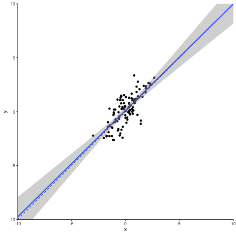
Simulated correlated normally distributed sample (n=100)
So, what happens when we disturb this statistical dream by changing one data point to become an outlier? We pick the data point that is closest to the distribution center and inflate its error term. This creates a ‘vertical outlier’, meaning a data point with a large absolute residual but which does not have an extreme value in terms of the independent variable(s). See the animation below for what a vertical outlier does to our regression.
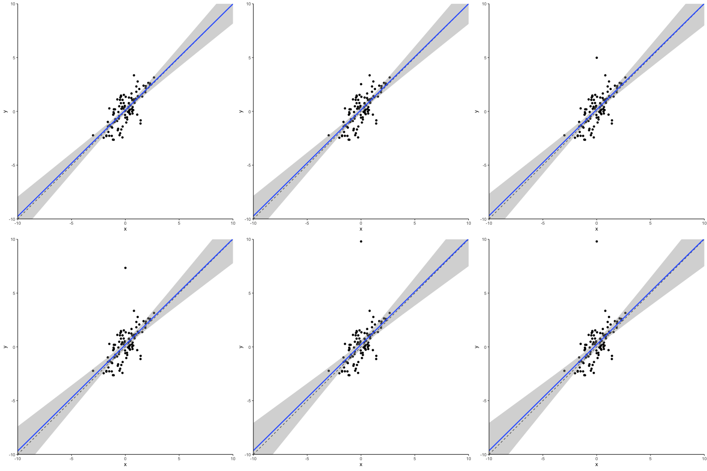
Vertical outlier
At first glance not much, you might say. But on closer inspection, you will see that as our courageous little outlier moves up vertically, the gray area highlighting the confidence interval of our regression estimates widens. This is what a vertical outlier does: it leaves the coefficient estimate unaffected but widens the standard errors, potentially making your precious regression table stars disappear.
Next let’s turn to another class of outliers, the so-called ‘leverage points’. They result from extreme values of independent variables. Depending on whether their corresponding dependent variable values reflect the underlying association or not, they can be characterized as either ‘good’ or ‘bad’. Good leverage points are located close to the unbiased regression line. They reduce the standard error (maybe even to an extent that can be considered too much) but they do not bias the coefficient. Let’s take a look at what a bad leverage point does to a regression.

Bad leverage point
Oops… This does not look good. A single observation is capable of tilting the regression line downwards, biasing it towards zero. Please note that this is the case here as our bad leverage point is strictly moving horizontally. If you have outliers that combine aspects of a vertical outlier and of a leverage point, then these can bias your coefficient up or down conditional on their location.
OK. Outliers can be bad for inference. How does robust regression help? To show you the intuition of how robust regression works, we simulated a sample that builds on the assumptions from above but contains a mixture of both vertical and horizontal outliers. Here it is along with a normal OLS regression line.
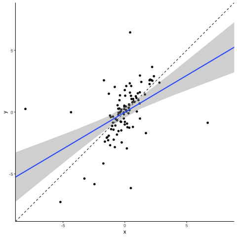
Outlier sample and OLS
You see that the outliers are doing their job. The regression line is clearly different from the correct 45° diagonal and the confidence interval is relatively wide. Robust regression to the rescue! The animation below tries to communicate the intuition on how robust regression works. It visualizes an M-estimator using a Huber loss function with a k value of 1.345 where the scale is being adjusted based on the median absolute deviation of the residuals. We throw all this detail at you so that you see that there is no such thing as “the robust regression method”. Robust regression approaches involve several design choices that you need to make and to communicate in your paper. If you are interested in more detail, read our paper, or maybe even better a good textbook on robust methods.
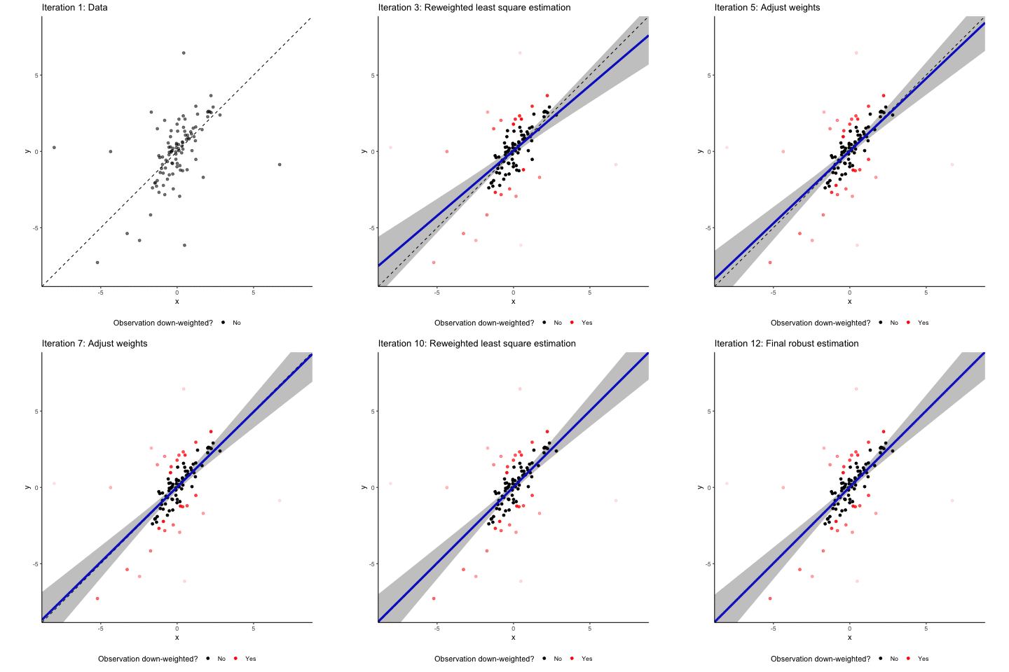
M Regression and iterated reweighted estimation
Back to the intuition. Robust regression involves several iterating steps where our sample observations are re-weighted. In a normal OLS, all observations enter into the estimation with a weight of one. The basic idea of robust regression is that you down-weight observations that have large absolute residuals. In the animation, these down-weighted observations are marked in red. The more they are down-weighted, the lighter they are plotted in the animation. After each reweighting, you (or your computer to be precise) generate(s) a new weighted estimate based on the new weights. This leads to new residuals based on which you can calculate new weights. These steps are repeated until the residuals do not change “much” anymore. You see that after these iterating steps, the resulting regression line is back to where it belongs: almost perfectly matching the 45° diagonal. Granted, we deliberately took an example where robust regression works very nicely. But rest assured that in a simulated setup like ours, robust regression methods are often well-suited to address the effect of random outliers on coefficient estimates.
Time to take this shiny method to some real data to see how it performs. Below you see a scatter plot of cash flow (cfo) and total accruals (tacc) data for a European sample of publicly listed non-financial firms (28,494 firm-year observations of Eurozone countries, covering the time period 2005 - 2019, data from Compustat Global). We follow the extant literature and scale both of these variables by firms’ average total assets. The vast majority of the data is bunched in the lower right corner of the graph. Clearly, as you can see below, the data contain extreme values for both the cash flow variable and the accrual variable that are much more extreme than our simulated data. Keep in mind that these data are deflated by average assets, meaning that a maximum value for tacc of more than 40 indicates that a firm has total accruals more than 40 times its average total assets. Wow!
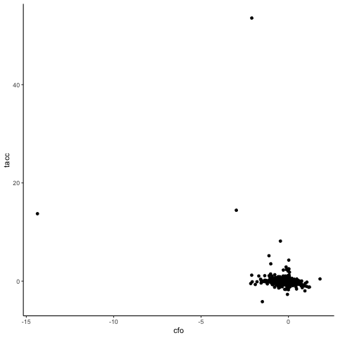
Accruals by Cashflows - unwinsorized
Let’s see how a robust regression estimator handles this dataset. For this, the animation below “zooms” in on the scatter plot by limiting the plotting area for each iteration step to observations that have a weight > 0.1.
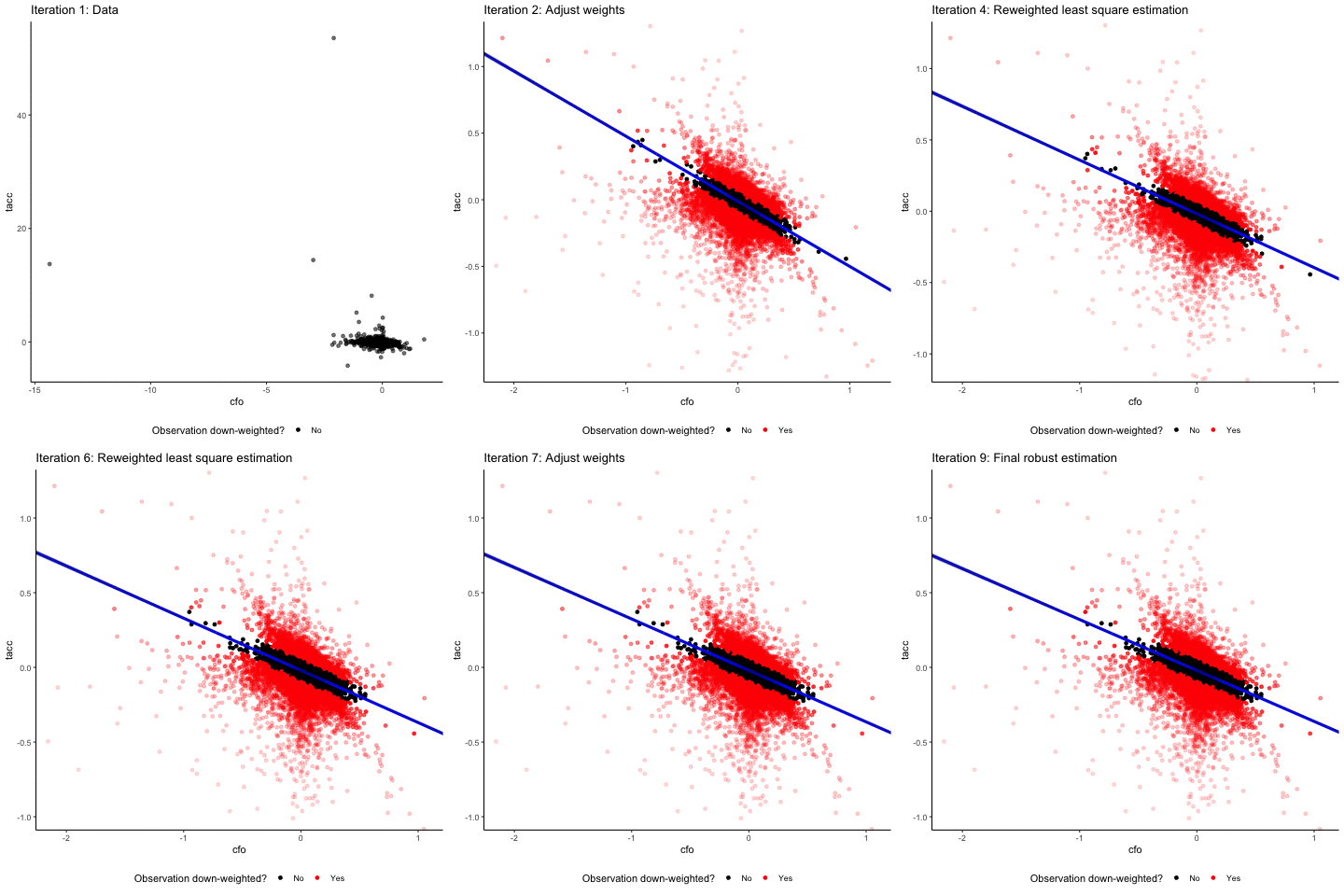
Accrual by Cashflows - Robust Regression
You see that, overall, the robust regression approach succeeds at down-weighting the extreme outliers and at focusing on the bulk of the data. You also see that the linear regression with the negative slope does not fit the data particularly well. We will come back to this later, but first we want to explore the nature of the outliers that our robust regression has identified a little bit.
First let’s see how the share of down-weighted observations compares across industries.
| Fama/French Industry | % down-weighted |
|---|---|
| Utilities | 7.0% |
| Chemicals and Allied Products | 20.4% |
| Consumer Durables | 20.9% |
| Wholesale, Retail, and Some Services | 21.0% |
| Consumer Non-durables | 22.2% |
| Manufacturing | 22.3% |
| Other | 24.6% |
| Oil, Gas, and Coal Extraction and Products | 26.6% |
| Business Equipment | 32.6% |
| Telephone and Television Transmission | 33.4% |
| Healthcare, Medical Equipment, and Drugs | 37.4% |
Now this does not look like a random distribution. Observations from intangible-intensive industries are much more likely to be down-weighted. What does the association of regression weights with size look like?
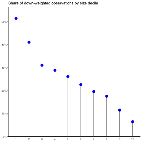
Robust weights by firm size
The smaller the firms, the more likely they are to get down-weighted and the smaller weights they receive. As a last test: is there also an association with sales growth? Yes!
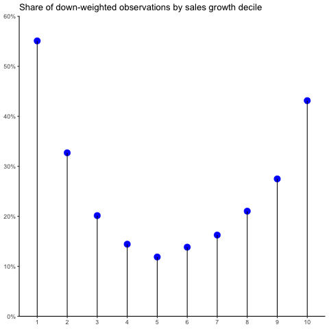
Robust weights by sales growth
You see: the smaller, the more intangible-intensive, and the more extreme in terms of growth firms are, the more likely they are to be down-weighted in our robust regression setup. This is a result of several aspects. While we discuss them in more detail in our working paper, here they are in a nutshell:
- Scaling by size introduces a mechanical association between size and the variance and skewness of variables;
- The economic nature of small and growing firms results in more extreme values;
- Intangible intensive firms have more extreme accounting treatments (i.e., here: no capitalization of intangible assets leads to large negative cash flows and low asset bases);
- Small firms are more likely to have limited data coverage and monitoring, resulting in a higher likelihood of data errors.
The implication of all this is that in an applied setting with non-random outliers, robust regression creates a sample selection bias. Depending on the research question at hand, this can be more or less problematic. To the very least, researchers should be aware of this bias and document and discuss it (see the end of this blog post for some suggestions on how to do this).
Next, we turn to our point “B” from above: The effect of misspecified regression models. While we use linear models in most of our settings, the association in the data is often not really linear. Sometimes, we have theoretical support for such non-linearity. In our case, for example, Ball and Shivakumar (JAR 2006) make a convincing case that, because of accounting conservatism, we can expect negative cash flows to have a less negative association with accruals than positive cash flows.
Why is this a problem for robust regression? Remember that it adjusts its weights according to the magnitude of the residuals, systematically down-weighting observations that are far away from the (potentially miss-specified) regression line. This causes the method to “zoom in” on the most dominant linear slope of the data, down-weighting any non-linearity present in the data. OLS instead fits its coefficients to reflect the average slope. This is an important difference. It is easy to overlook non-linearities when you use robust regression.
To visualize this problem, let’s look at a final simulation (we promise!). Below you see a plot of a polynomial of the type y = x^3 + x^2 + x. We sampled 100 data points from a normal x (mean = 0, variance = 1) and added an independently normal distributed error term (again, mean = 0, variance = 1) to calculate y. You see that the OLS regression picks up some of the steeper slopes of the extremes.
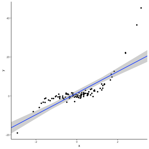
Simulation of a non-linear association with OLS (n = 100)
Now let’s see what the iterated reweighted estimation approach of the robust regression does to the same data. You notice that it, consistent with the misspecified linear form of the regression model, systematically down-weights the extreme observations. This results in a significant decline in slope, essentially fitting the model to the central bulk of the data, disguising the prominent non-linearity in the data.
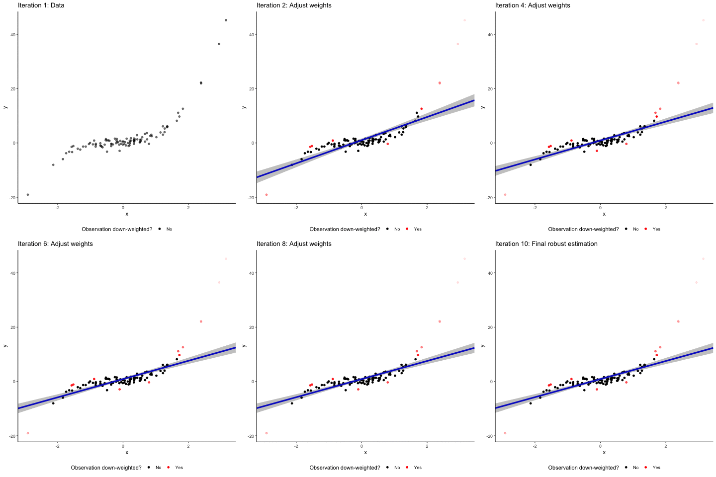
Non-linear association and robust regression
Of course, you might argue that this effect is driven by the specific sample having rather extreme observations. To show you that this indeed is a systematic issue, we repeat the exercise 100 times and compare the OLS and M-estimator coefficients. In the plot below, the blue lines indicate OLS and the red lines robust regressions. You can instantly see that robust regressions have smaller slopes on average, down-weighting the effect of the non-linearity.
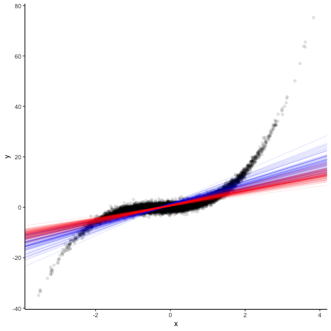
100 regressions - OLS and robust
Now how does this affect our analysis of the cash flow-accrual relation? To see this, we first take a “traditional” approach and estimate a linear model based on OLS for a sample with winsorized data. We then compare these regression results (blue line) with those that we get from a robust regression based on non-winsorized data (red line).
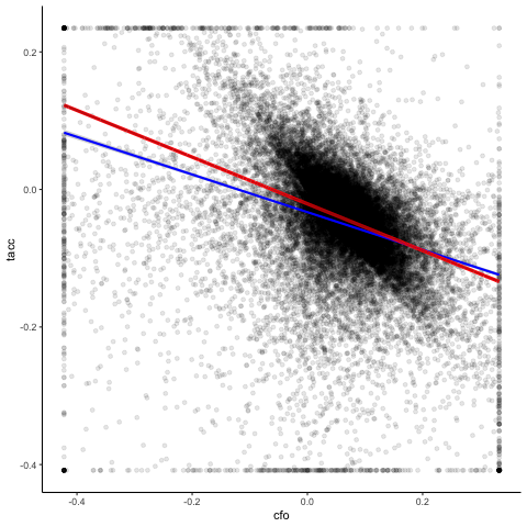
Accruals by cashflows - linear OLS and RR
You see a clear difference between the two regressions. The robust red line is more downward sloping than the blue line from the OLS estimation. When instead of a normal linear model, we estimate a Ball-Shivakumar interacted model that allows different slopes and intercepts for negative and positive cash flow observations, we get the following result.
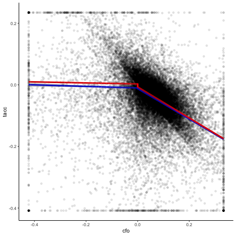
Accruals by cashflows - interacted OLS and RR
You see for this specification that robust regression of the untreated data and OLS based on winsorized data yield almost identical results. Thus, the differences between the robust regression and OLS results above were not driven by outliers biasing OLS, but by model misspecification affecting both approaches differently. While for OLS, the linear coefficient is a weighted average of the negative and positive slopes, the robust regression approach puts more weight on positive cash flow observations and biases the coefficient downwards.
We hope that the above was helpful to you to understand our three main points: (A) Outliers are almost always not random, (B) models are often misspecified and thus, (C) we can expect robust regression to yield biased estimates in applied settings. Does this mean that we should discard robust regression and instead return to running OLS with arbitrary outlier treatments? No! In most applied settings, estimates will be biased regardless of the method used. A careful researcher should be aware of these biases and trade off method efficiency with bias, as well as communicate the advantages and disadvantages of a certain method choice to the reader in an understandable way.
So, here are our suggestions on how to deal with outliers like a pro. The following is based on the assumption that you already have a prediction that you want to test and the required data for it in mind.
Step 1: Explore!
- Before looking at your data, sketch the distributions you expect it to have. These predictions should be based on your understanding of the underlying economics, the data generating process, and the way you defined and calculated your variables.
- Verify your assumptions by visual inspection (histograms, kernel density plot) and by tabulating descriptive statistics of your variables. Don’t forget the higher moments: Skewness will tell you whether your distribution is right-skewed (positive skewness, like most size-related measures) or left-skewed (negative skewness). Kurtosis measures the heaviness of the tails. A normal distribution has a Kurtosis of three, unwinsorized accounting data can have Kurtosis values > 1,000!
- Verify whether your causal thinking from above is correct. This means that you need to look at some extreme data points to verify that they are extreme for the reason that you expected before looking at the data.
- Often, you will identify issues that will make you reconsider your thought process and maybe also change the way you construct your variables. Possible remedies are transformation using for example the log function, scaling, or ranking (in deciles or maybe even into a binary variable).
- After assessing the univariate distributions of your variables, it is time to identify your outliers multivariately. Again, a first good step is to visualize the associations of your data (scatter plots, two-dimensional density plots, correlation matrices).
- Then, estimate a robust regression model and store the weights. Remember: down-weighted observations identify outliers.
- Explore the non-random nature of these outliers by contrasting the descriptive statistics of the weighted sample with the unweighted sample. For this purpose, you can use the robust balance table that we introduce in our paper.
- Also verify whether the identified outliers are indicative of nonlinearities with regards to the main association of interest. This can easily be done by plotting weights against your main variable of interest. Non-random patterns are indicative of potential unmodeled non-linearities.
Step 2: Estimate!
- After exploring the nature of your data univariately and multivariately, you are ready to get to work and select the estimation method that best fits your theory and your data.
- If your outliers appear to be random and are not indicative of non-linearities in the underlying association of interest, robust regression approaches are a good idea. To keep traditionalists happy, you could report findings from winsorized. approaches along with them. They should not vary a lot, anyway. See the online appendix of our paper for advice on how to deal with fixed effects and clustered standard errors.
- If your outliers are non-random, document this non-randomness with the robust balance table mentioned above.
- If the outliers are clustered in a part of a sample that you care about, it might be a good idea to prepare some subsample analysis focused on the outliers, maybe using locally weighted regression.
- If your outliers are indicative of non-linearities in the underlying association of interest, consider addressing this non-linearity in your model design, for example by using piecewise regression, higher order polynomials, or locally smoothed regression approaches.
- If you cannot decide between alternatives or to explain how your design choice affects your findings (see below), you can also report multiple estimation results side-by-side, either in a table, in a coefficient plot, or, if you have many different specifications, by using a specification curve.
Step 3: Explain!
- To document and discuss your analysis, you can use any subset from the tables and visuals mentioned above. We recommend combining visuals that reflect the multivariate association of interest with a robust balance table that documents the effect of outliers on the data and the discrepancies between the original sample and the sample used in the robust analysis.
- Every research design choice comes with benefits and costs attached and outlier treatments are clearly no exception. You can make the life of your readers much easier by discussing your methodological trade-offs in non-technical jargon and focusing on the research question. So, consider replacing the standard “To reduce the impact of outliers on our findings, we winsorize the dependent and independent variables at the top and bottom percentile” with “In our data, small firms, firms from intangible intensive industries and firms that have extreme growth patterns are significantly more likely to generate outlier observations. To limit their influence on our main tests, we use robust regression estimators. After addressing the inherent non-linearity in our data, the resulting findings are largely identical to using traditional winsorizing and are robust across various design choices. Based on this, we conclude that they fairly represent the average effect for the majority of our sample, but we caution the reader when generalizing our findings to small firms, extreme growth firms, and firms from intangible intensive industries.”
Link to the paper on SSRN: https://papers.ssrn.com/sol3/papers.cfm?abstract_id=3880942 Link to the Github page containing the analyses of this blog post and relevant programs: https://github.com/dveenman/outliers
