Exploring and Benchmarking Oxford Government Response Data
Exploring and Benchmarking Oxford Government Response Data
Assessing the impact of Non-Pharmaceutical Interventions on the spread of Covid-19 requires data on Governmental measures. Luckily, the Assessment Capacities Project (ACAPS) and the Oxford Covid-19 Government Response Tracker both provide such data. In this blog post, I explore the new data provided by the Oxford initiative and compare it against the data provided by ACAPS that is already included in my {tidycovid19} package that offers download handles and some visualization tools for Covid-19 related data.
The publication of the Governance Tracker Data has spurred some interest by the media and the academic community and there are already studies using it. Its methodology is being presented in Hale, Thomas, Anna Petherick, Toby Phillips, Samuel Webster. “Variation in Government Responses to COVID-19” Version 3.0. Blavatnik School of Government Working Paper. March 31, 2020.
Downloading and data cleaning
Downloading the data form the Oxford homepage is straightforward. Automatic column detection by read_xlsx() fails so I provide columns manually.
suppressPackageStartupMessages({
  library(kableExtra)
  library(dplyr)
  library(tidyr)
  library(lubridate)
  library(tidycovid19)
  library(ggplot2)
  library(stringr)
  library(readxl)
  library(gghighlight)
  library(RCurl)
})

dta_url <- "https://www.bsg.ox.ac.uk/sites/default/files/OxCGRT_Download_latest_data.xlsx"
tmp_file <- tempfile(".xlsx")
utils::download.file(dta_url, tmp_file, mode = "wb")

raw_data <- read_xlsx(
  tmp_file,
  col_types = c("text", "text", "numeric",
                rep(c("numeric", "numeric", "text"), 6),
                rep(c("numeric", "text"), 5), rep("numeric", 3), "skip")
)
The file is organized by country-date and sorted by date. As in essence interventions data is event driven for each country (meaning that interventions happen infrequently at certain dates), I sort the data by country-date to get a better view on its structure. Also, I adjust some names and concentrate on the policy measures first, discarding the other data for the time being.
raw_data <- raw_data %>%
  dplyr::rename(
    country = CountryName,
    iso3c = CountryCode,
    date = Date
  ) %>%
  dplyr::mutate(date = lubridate::ymd(date)) %>%
  arrange(iso3c, date)

df <- raw_data %>%
  select(-country, -ConfirmedCases, -ConfirmedDeaths, -ends_with("_Notes"),
         -ends_with("_IsGeneral"), -StringencyIndex,
         -starts_with(paste0("S", 8:11)))

kable(df %>% head(20)) %>% kable_styling()| iso3c | date | S1_School closing | S2_Workplace closing | S3_Cancel public events | S4_Close public transport | S5_Public information campaigns | S6_Restrictions on internal movement | S7_International travel controls |
|---|---|---|---|---|---|---|---|---|
| ABW | 2020-03-13 | NA | NA | NA | NA | NA | NA | NA |
| ABW | 2020-03-15 | NA | NA | NA | NA | NA | NA | 3 |
| ABW | 2020-03-16 | 2 | NA | 2 | NA | NA | NA | 3 |
| ABW | 2020-03-17 | 2 | NA | 2 | NA | NA | NA | 3 |
| ABW | 2020-03-18 | 2 | NA | 2 | NA | NA | NA | 3 |
| ABW | 2020-03-19 | 2 | NA | 2 | NA | NA | NA | 3 |
| ABW | 2020-03-20 | 2 | NA | 2 | NA | NA | NA | 3 |
| ABW | 2020-03-21 | 2 | NA | 2 | NA | NA | 2 | 3 |
| ABW | 2020-03-22 | 2 | NA | 2 | NA | NA | 2 | 3 |
| ABW | 2020-03-23 | 2 | NA | 2 | NA | NA | 2 | 3 |
| ABW | 2020-03-24 | 2 | NA | 2 | NA | NA | 2 | 3 |
| ABW | 2020-03-25 | 2 | NA | 2 | NA | NA | 2 | 3 |
| ABW | 2020-03-26 | 2 | NA | 2 | NA | NA | 2 | 3 |
| ABW | 2020-03-27 | 2 | NA | 2 | NA | NA | 2 | 3 |
| ABW | 2020-03-28 | 2 | NA | 2 | NA | NA | 2 | 3 |
| ABW | 2020-03-29 | 2 | NA | 2 | NA | NA | 2 | 3 |
| ABW | 2020-03-30 | 2 | NA | 2 | NA | NA | 2 | 3 |
| ABW | 2020-03-31 | 2 | NA | 2 | NA | NA | 2 | 3 |
| AFG | 2020-01-01 | 0 | NA | 0 | NA | 0 | 0 | 0 |
| AFG | 2020-01-02 | 0 | NA | 0 | NA | 0 | 0 | 0 |
You can see that at some point of time measures are introduced and then they are maintained. To make it more transparent which events are actually driving the values, I reorganize the data into an country-date-npi_type structure. This requires some shuffling and tidying as each NPI type has three variables and the actual type is captured in a variable name.
df <- raw_data

# Fix column names for pivot_long()
names(df)[seq(from = 4, by = 3, length.out = 7)] <- paste0("S", 1:7, "_measure")


df <- df %>% select(1:23) %>%
# S7 has no "IsGeneral" value. I attach an NA var for consistency
  mutate(S7_IsGeneral = NA) %>%
  pivot_longer(4:24, names_pattern = "(.*)_(.*)", names_to = c("type", ".value")) %>%
  rename(npi_measure = measure, npi_is_general = IsGeneral, npi_notes = Notes)

# Fix NPI type categories
lup <- tibble(
  type = paste(paste0("S", 1:7)),
  npi_type = sub("S\\d*_", "", names(raw_data)[seq(from = 4, by = 3, length.out = 7)])
)

oxford_pm <- df %>%
  left_join(lup, by = "type") %>%
  select(iso3c, country, date, npi_type, npi_measure, npi_is_general, npi_notes) %>%
  arrange(iso3c, npi_type, date)

# Let'#'s display an example

oxford_pm %>%
  filter(iso3c == "ABW" & npi_type == "Restrictions on internal movement") %>%
kable() %>% kable_styling() | iso3c | country | date | npi_type | npi_measure | npi_is_general | npi_notes |
|---|---|---|---|---|---|---|
| ABW | Aruba | 2020-03-13 | Restrictions on internal movement | NA | NA | NA |
| ABW | Aruba | 2020-03-15 | Restrictions on internal movement | NA | NA | NA |
| ABW | Aruba | 2020-03-16 | Restrictions on internal movement | NA | NA | NA |
| ABW | Aruba | 2020-03-17 | Restrictions on internal movement | NA | NA | NA |
| ABW | Aruba | 2020-03-18 | Restrictions on internal movement | NA | NA | NA |
| ABW | Aruba | 2020-03-19 | Restrictions on internal movement | NA | NA | NA |
| ABW | Aruba | 2020-03-20 | Restrictions on internal movement | NA | NA | NA |
| ABW | Aruba | 2020-03-21 | Restrictions on internal movement | 2 | NA |
Curfew set (9PM until 6AM). Violations can be met with fines up to AWG 10,000 (over US$5000). Shops need to be closed by 8PM every day. https://www.overheid.aw/actualidad/noticia_47171/item/decisionnan-tuma-pa-gobierno-relaciona-cu-e-crisis-di-coronavirus-covid-19_48506.html |
| ABW | Aruba | 2020-03-22 | Restrictions on internal movement | 2 | NA |
Curfew set (9PM until 6AM). Violations can be met with fines up to AWG 10,000 (over US$5000). Shops need to be closed by 8PM every day. https://www.overheid.aw/actualidad/noticia_47171/item/decisionnan-tuma-pa-gobierno-relaciona-cu-e-crisis-di-coronavirus-covid-19_48506.html |
| ABW | Aruba | 2020-03-23 | Restrictions on internal movement | 2 | NA |
Curfew set (9PM until 6AM). Violations can be met with fines up to AWG 10,000 (over US$5000). Shops need to be closed by 8PM every day. https://www.overheid.aw/actualidad/noticia_47171/item/decisionnan-tuma-pa-gobierno-relaciona-cu-e-crisis-di-coronavirus-covid-19_48506.html |
| ABW | Aruba | 2020-03-24 | Restrictions on internal movement | 2 | NA |
Curfew set (9PM until 6AM). Violations can be met with fines up to AWG 10,000 (over US$5000). Shops need to be closed by 8PM every day. https://www.overheid.aw/actualidad/noticia_47171/item/decisionnan-tuma-pa-gobierno-relaciona-cu-e-crisis-di-coronavirus-covid-19_48506.html |
| ABW | Aruba | 2020-03-25 | Restrictions on internal movement | 2 | NA |
Curfew set (9PM until 6AM). Violations can be met with fines up to AWG 10,000 (over US$5000). Shops need to be closed by 8PM every day. https://www.overheid.aw/actualidad/noticia_47171/item/decisionnan-tuma-pa-gobierno-relaciona-cu-e-crisis-di-coronavirus-covid-19_48506.html |
| ABW | Aruba | 2020-03-26 | Restrictions on internal movement | 2 | NA |
Curfew set (9PM until 6AM). Violations can be met with fines up to AWG 10,000 (over US$5000). Shops need to be closed by 8PM every day. https://www.overheid.aw/actualidad/noticia_47171/item/decisionnan-tuma-pa-gobierno-relaciona-cu-e-crisis-di-coronavirus-covid-19_48506.html |
| ABW | Aruba | 2020-03-27 | Restrictions on internal movement | 2 | NA |
Curfew set (9PM until 6AM). Violations can be met with fines up to AWG 10,000 (over US$5000). Shops need to be closed by 8PM every day. https://www.overheid.aw/actualidad/noticia_47171/item/decisionnan-tuma-pa-gobierno-relaciona-cu-e-crisis-di-coronavirus-covid-19_48506.html |
| ABW | Aruba | 2020-03-28 | Restrictions on internal movement | 2 | NA |
Curfew set (9PM until 6AM). Violations can be met with fines up to AWG 10,000 (over US$5000). Shops need to be closed by 8PM every day. https://www.overheid.aw/actualidad/noticia_47171/item/decisionnan-tuma-pa-gobierno-relaciona-cu-e-crisis-di-coronavirus-covid-19_48506.html |
| ABW | Aruba | 2020-03-29 | Restrictions on internal movement | 2 | NA |
Curfew set (9PM until 6AM). Violations can be met with fines up to AWG 10,000 (over US$5000). Shops need to be closed by 8PM every day. https://www.overheid.aw/actualidad/noticia_47171/item/decisionnan-tuma-pa-gobierno-relaciona-cu-e-crisis-di-coronavirus-covid-19_48506.html |
| ABW | Aruba | 2020-03-30 | Restrictions on internal movement | 2 | NA |
Curfew set (9PM until 6AM). Violations can be met with fines up to AWG 10,000 (over US$5000). Shops need to be closed by 8PM every day. https://www.overheid.aw/actualidad/noticia_47171/item/decisionnan-tuma-pa-gobierno-relaciona-cu-e-crisis-di-coronavirus-covid-19_48506.html |
| ABW | Aruba | 2020-03-31 | Restrictions on internal movement | 2 | NA |
Curfew set (9PM until 6AM). Violations can be met with fines up to AWG 10,000 (over US$5000). Shops need to be closed by 8PM every day. https://www.overheid.aw/actualidad/noticia_47171/item/decisionnan-tuma-pa-gobierno-relaciona-cu-e-crisis-di-coronavirus-covid-19_48506.html |
In this snippet of the data everything is sticky, even the notes. To remove these stale data from the sample, I next limit the sample to observations that differ from the country-day before. First rows are only kept if they contain non-missing data. Note that this does not discard information. It just helps making the data more parsimonious. Just compare the information on Aruba after the cleaning with the one above.
oxford_pm_events <- oxford_pm %>%
  group_by(iso3c, npi_type) %>%
  filter(
    (row_number() == 1 &
       (!is.na(npi_is_general) | !is.na(npi_measure) | !is.na(npi_notes)))  |
      (is.na(lag(npi_is_general)) & !is.na(npi_is_general)) |
      (is.na(lag(npi_measure)) & !is.na(npi_measure)) |
      (is.na(lag(npi_notes)) & !is.na(npi_notes)) |
      (!is.na(lag(npi_is_general)) & is.na(npi_is_general)) |
      (!is.na(lag(npi_measure)) & is.na(npi_measure)) |
      (!is.na(lag(npi_notes)) & is.na(npi_notes)) |
      (lag(npi_is_general) != npi_is_general) |
      (lag(npi_measure) != npi_measure) |
      (lag(npi_notes) != npi_notes)
  ) %>%
  ungroup()

oxford_pm_events %>%
  filter(iso3c == "ABW" & npi_type == "Restrictions on internal movement") %>%
kable() %>% kable_styling() | iso3c | country | date | npi_type | npi_measure | npi_is_general | npi_notes |
|---|---|---|---|---|---|---|
| ABW | Aruba | 2020-03-21 | Restrictions on internal movement | 2 | NA |
Curfew set (9PM until 6AM). Violations can be met with fines up to AWG 10,000 (over US$5000). Shops need to be closed by 8PM every day. https://www.overheid.aw/actualidad/noticia_47171/item/decisionnan-tuma-pa-gobierno-relaciona-cu-e-crisis-di-coronavirus-covid-19_48506.html |
When you go through the data in this format you will spot a set of minor inconsistencies:
- Most of the time, notes are only added on the event date but sometimes, like in the example above for Aruba, they are stale. This makes it harder to identify redundant data.
- Some countries are “initialized” with 0 values for some measures while others are not. I am not sure whether this difference is substantiated by data (most of these cases do not have notes, see below) or whether it is an artifact of data collection.
- There are quite a few observations with zero measures that are classified as ‘general’ or not regardless. I am also not sure what this implies.
- There are missing observations for some countries in recent dates, breaking the general principle that stale but still in-place measures are normally just written forward.
- Many references in the notes variables are not authoritative even if authoritative resources should exist (more on this below).
Are there any odd cases?
Potentially odd cases could be where measures decrease over time. Let’s do a quick sanity check
oxford_pm_events %>%
  group_by(iso3c, npi_type) %>%
  filter(lead(npi_measure) < npi_measure | lag(npi_measure) > npi_measure) -> df

nrow(df)
## [1] 96# Example Mexico
df %>%
filter(iso3c == "MEX") %>%
kable() %>% kable_styling() | iso3c | country | date | npi_type | npi_measure | npi_is_general | npi_notes |
|---|---|---|---|---|---|---|
| MEX | Mexico | 2020-03-14 | Cancel public events | 1 | 1 | March 14, The Health Secretariat recommends to keep a “healthy distance” and avoid non-essential working, starting on 23 of Ma |
| MEX | Mexico | 2020-03-15 | Cancel public events | 0 | 0 | NA |
| MEX | Mexico | 2020-02-07 | International travel controls | 3 | NA | NA |
| MEX | Mexico | 2020-03-18 | International travel controls | 1 | NA | NA |
| MEX | Mexico | 2020-03-14 | School closing | 1 | 1 | March 14, the Public Education Secretariat suspends classes from 23 of March until 19 of April. [https://www.gob.mx/salud/pren |
| MEX | Mexico | 2020-03-15 | School closing | 0 | 0 | NA |
| MEX | Mexico | 2020-03-17 | School closing | 2 | 0 | Although the national recommendation is to close schools until March 20, as Mexico is a Federation, some states have decided t |
| MEX | Mexico | 2020-03-18 | School closing | 0 | 1 | NA |
| MEX | Mexico | 2020-03-14 | Workplace closing | 1 | 1 | March 14, The Health Secretariat recommends to keep a “healthy distance” and avoid non-essential working, starting on 23 of Ma |
| MEX | Mexico | 2020-03-15 | Workplace closing | 0 | 0 | NA |
While many of those cases seem to be supported by notes and are thus likely to consistent, the Mexican example shows a recurrent pattern: Sometimes measures are seemingly “revoked” just one day later with no note supporting the data. This could be an artifact of accidentally mixing level measures with event measures. In addition, it appears the notes are truncated and they seem to indicate that the measures were meant to be effective on March 23, a fact that is not captured in the data.
Comparing number of interventions and notes coverage with ACAPS data
Because of the above mentioned inconsistencies in the data, assessing the actual number of coded interventions is non-trivial. I assume that an intervention is defined either by a note that is only attached to a specific date (but not to the date before or after) or by a change in the measurement.
oxford_pm_events %>%
  group_by(iso3c, npi_type) %>%
  filter((row_number() == 1 )|
           (lag(npi_measure) != npi_measure) |
           (lag(npi_is_general) != npi_is_general) |
           (!is.na(npi_notes) & (lag(npi_notes) != npi_notes))) %>%
  mutate(notes_avail = !is.na(npi_notes)) %>%
  ungroup() -> ope

addmargins(table(ope$npi_type, ope$notes_avail))
##
## FALSE TRUE Sum
## Cancel public events 101 144 245
## Close public transport 83 79 162
## International travel controls 94 266 360
## Public information campaigns 85 136 221
## Restrictions on internal movement 91 138 229
## School closing 96 160 256
## Workplace closing 93 136 229
## Sum 643 1059 1702acaps_df <- download_acaps_npi_data(cached = TRUE, silent = TRUE) %>%
mutate(notes_avail = !is.na(link))
addmargins(table(acaps_df$category, acaps_df$notes_avail))##
## FALSE TRUE Sum
## Humanitarian exemption 0 2 2
## Lockdown 0 102 102
## Movement restrictions 7 948 955
## Public health measures 3 1086 1089
## Social and economic measures 1 520 521
## Social distancing 6 702 708
## Sum 17 3360 3377The ACAPS data has 60 % more interventions and almost full coverage with sources. In the Oxford dataset, currently roughly 60 % of the identified interventions are backed with sources but this might well be an artifact of my intervention identification approach.
Let’s see how source coverage varies by be measurement magnitude for the Oxford data.
addmargins(table(ope$npi_measure, ope$notes_avail))##
## FALSE TRUE Sum
## 0 584 35 619
## 1 30 374 404
## 2 26 531 557
## 3 3 116 119
## Sum 643 1056 1699This seems to be the case. The “zero measures” have only rarely notes attached. The non-zero measures look much better in terms of coverage. Yet another reason not to use the zero measures.
How does the quality of the notes compare? To get an idea about this I compare the urls included in the notes for the Mexican cases
url_pattern <- "http[s]?://(?:[a-zA-Z]|[0-9]|[$-_@.&+]|[!*\\(\\),]|(?:%[0-9a-fA-F][0-9a-fA-F]))+"

ope %>%
  mutate(link = str_extract(npi_notes, url_pattern)) %>%
  select(iso3c, date, link) %>% na.omit() %>%
  arrange(date) -> oxford_urls

oxford_urls %>%
  filter(iso3c == "MEX") %>%
  select(-iso3c) %>%
kable() %>% kable_styling() bind_rows(
acaps_df %>%
mutate(date = as_date(date_implemented)) %>%
select(iso3c, date, link),
acaps_df %>%
select(iso3c, date_implemented, `alternative source`) %>%
mutate(date = as_date(date_implemented)) %>%
rename(link = `alternative source`) %>%
select(-date_implemented)
) %>%
mutate(link = str_extract(link, url_pattern)) %>%
na.omit() %>%
arrange(date) -> acaps_urls
acaps_urls %>%
filter(iso3c == "MEX") %>%
select(-iso3c) %>%
kable() %>% kable_styling() You see that some of the Oxford URLs seem truncated and most do not point to governmental resources directly while the ACAPS URLs all seem to link to authoritative sources. Last check on this. How many URLs return an OK header, meaning that they can be reached but not necessarily that they will still return the required data. I test this on a sample of 100 URls from both sources.
return_pct_valid_urls <- function(df, n = 100) {
  urls <- df %>% sample_n(n) %>% pull(link)
  works <- sapply(urls, url.exists)
  sum(works)/n
}

return_pct_valid_urls(oxford_urls, 100)
## [1] 0.81return_pct_valid_urls(acaps_urls, 100)## [1] 0.94It appears that the source URLs provided by ACAPS are in better shape. Time to compare the two data sources in terms of actual measures. Let’s first look at the coverage across countries.
acaps <- download_acaps_npi_data(cached = TRUE, silent = TRUE)
acaps %>% select(iso3c) %>% unique() %>% nrow()
## [1] 182raw_data %>% select(iso3c) %>% unique() %>% nrow()## [1] 190oxford_pm_events %>% filter(npi_measure > 0) %>% select(iso3c) %>% unique() %>% nrow()## [1] 90The ACAPS data covers a much wider array of countries but the Oxford data also spans an impressive list of countries. While their raw data file contains 190 country identifiers it seems to contain actual data currently for 90 countries. In their documentation, the team states that they have collected data for 77 countries but that they plan to enlarge their sample.
To compare the intervention measures themselves, as the categories are not comparable, I compare a ranked measure of the appropriate ACAPS measures with the Stringency Measure of the Oxford data.
 download_merged_data(cached = TRUE, silent = TRUE) %>%
  mutate(acaps_score = 100*((soc_dist/max(soc_dist, na.rm = TRUE) +
           mov_rest/max(mov_rest, na.rm = TRUE) + lockdown)/3)) %>%
  mutate(acaps_score = 100*percent_rank(acaps_score)) %>%
  left_join(raw_data %>%
              rename(oxford_si = StringencyIndex) %>%
              select(iso3c, date, oxford_si),
            by = c("iso3c", "date"))  %>%
  select(iso3c, date, acaps_score, oxford_si) -> df

summary(df)
## iso3c date acaps_score oxford_si
## Length:12994 Min. :2020-01-22 Min. : 0.00 Min. : 0.00
## Class :character 1st Qu.:2020-02-09 1st Qu.: 0.00 1st Qu.: 0.00
## Mode :character Median :2020-02-27 Median : 0.00 Median : 14.00
## Mean :2020-02-27 Mean :30.37 Mean : 24.35
## 3rd Qu.:2020-03-16 3rd Qu.:74.51 3rd Qu.: 38.00
## Max. :2020-04-03 Max. :99.98 Max. :100.00
## NA's :7639df %>%
pivot_longer(3:4, names_to = "source", values_to = "measure") %>%
filter(!is.na(measure)) %>%
group_by(date, source) %>%
summarize(
mn = mean(measure),
se = sd(measure)/sqrt(n())
) %>%
ggplot(aes(x = date, y = mn, color = source)) +
geom_pointrange(
aes(ymin = mn-1.96*se, ymax = mn+1.96*se),
position=position_dodge(0.4)
)
df %>%
  filter(!is.na(oxford_si) & !is.na(acaps_score)) %>%
  group_by(iso3c) %>%
  summarise(oxford_si = mean(oxford_si),
            acaps_score = mean(acaps_score)) %>%
  ggplot(aes(x = oxford_si, y = acaps_score)) + geom_point() +
  gghighlight(abs(oxford_si - acaps_score) > 30, label_key = iso3c)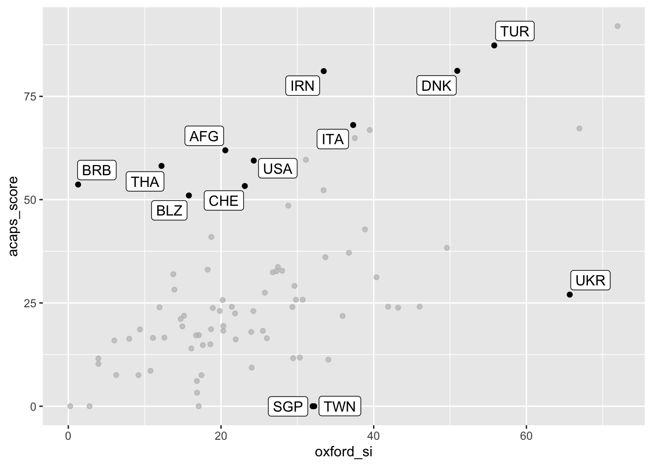
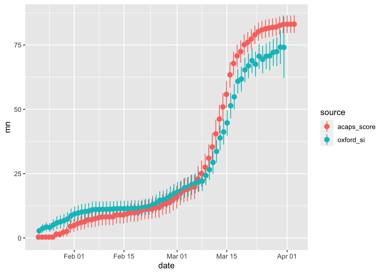
The two measures are clearly correlated but it also becomes apparent that the country-level averages vary significantly. Thus, it seems likely that the choice of the data source might have an impact on research findings.
Replicating the Oxford Government Response Stringency Index
The team of the Oxford Blavatnik School has constructed an aggregate “stringency” measure. Many people will be tempted to use this measure as an overall indicator for the country-level intensity of interventions. Thus, I try to reproduce this measure to assess its internal validity.
From the working paper documenting the dataset:
Our baseline measure of variation in governments’ responses is the COVID-19 Government Response Stringency Index (Stringency Index). For each ordinal policy response measure S1-S7, we create a score by taking the ordinal value and adding one if the policy is general rather than targeted, if applicable. This creates a score between 0 and 2 and for S5, and 0 and 3 for the other six responses. We then rescale each of these by their maximum value to create a score between 0 and 100, with a missing value contributing 0. These seven scores are then averaged to get the composite Stringency Index.
I implement this approach using the original data
si <- oxford_pm %>%
  group_by(iso3c, date) %>%
  summarise(delete = all(is.na(npi_measure)) & all(is.na(npi_is_general))) %>%
  left_join(oxford_pm, by = c("iso3c", "date")) %>%
  filter(!delete) %>%
  select(-delete) %>%
  mutate(
    npi_measure = replace_na(npi_measure, 0),
    npi_is_general = replace_na(npi_is_general, 0)
  ) %>%
  group_by(npi_type) %>%
  mutate(score = (npi_measure + npi_is_general)/max(npi_measure + npi_is_general)) %>%
  group_by(iso3c, date) %>%
  summarise(si_100 = round(100*mean(score)))

df <- raw_data %>% select(iso3c, date, StringencyIndex) %>%
  left_join(si, by = c("iso3c", "date"))

summary(df)
## iso3c date StringencyIndex si_100
## Length:10561 Min. :2020-01-01 Min. : 0.00 Min. : 0.00
## Class :character 1st Qu.:2020-01-26 1st Qu.: 0.00 1st Qu.: 0.00
## Mode :character Median :2020-02-20 Median : 5.00 Median : 10.00
## Mean :2020-02-18 Mean : 19.59 Mean : 20.68
## 3rd Qu.:2020-03-15 3rd Qu.: 29.00 3rd Qu.: 29.00
## Max. :2020-03-31 Max. :100.00 Max. :100.00
## NA's :3280 NA's :3046ggplot(df, aes(x = StringencyIndex, y = si_100)) +
geom_point(alpha = 0.2) + theme_minimal()## Warning: Removed 3280 rows containing missing values (geom_point).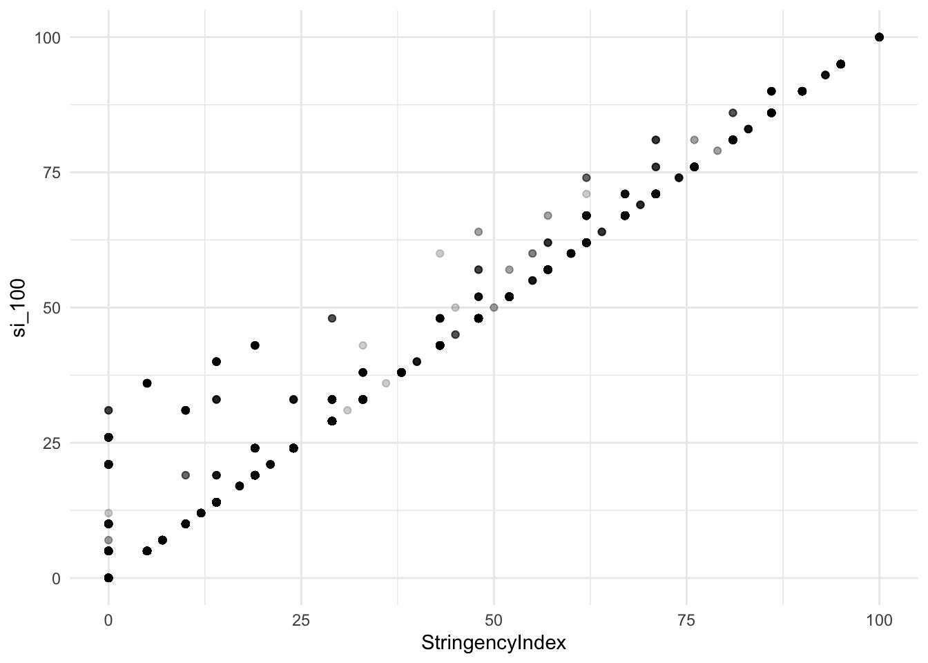
Not all observations have identical values. There is a substantial amount of data where my reproduced measure has higher values compared to the measure reported by the Oxford team. After inspecting the data I got the impression that the Oxford team does not add the ‘is_general’ value when the ‘measure’ value for a certain intervention is zero. Testing this conjecture yields the following.
si <- oxford_pm %>%
  group_by(iso3c, date) %>%
  summarise(delete = all(is.na(npi_measure)) & all(is.na(npi_is_general))) %>%
  left_join(oxford_pm, by = c("iso3c", "date")) %>%
  filter(!delete) %>%
  select(-delete) %>%
  mutate(
    npi_measure = replace_na(npi_measure, 0),
    npi_is_general = replace_na(npi_is_general, 0)
  ) %>%
  group_by(npi_type) %>%
  mutate(score = ifelse(npi_measure > 0,
                        npi_measure + npi_is_general,
                        npi_measure)/max(npi_measure + npi_is_general)) %>%
  group_by(iso3c, date) %>%
  summarise(si_100 = round(100*mean(score)))

df <- raw_data %>% select(iso3c, date, StringencyIndex) %>%
  left_join(si, by = c("iso3c", "date"))

summary(df)
## iso3c date StringencyIndex si_100
## Length:10561 Min. :2020-01-01 Min. : 0.00 Min. : 0.00
## Class :character 1st Qu.:2020-01-26 1st Qu.: 0.00 1st Qu.: 0.00
## Mode :character Median :2020-02-20 Median : 5.00 Median : 5.00
## Mean :2020-02-18 Mean : 19.59 Mean : 19.43
## 3rd Qu.:2020-03-15 3rd Qu.: 29.00 3rd Qu.: 29.00
## Max. :2020-03-31 Max. :100.00 Max. :100.00
## NA's :3280 NA's :3046ggplot(df, aes(x = StringencyIndex, y = si_100)) +
geom_point(alpha = 0.2) + theme_minimal() ## Warning: Removed 3280 rows containing missing values (geom_point).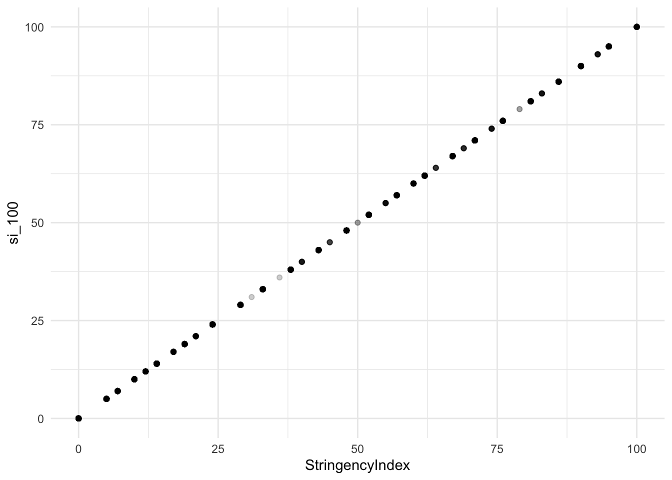
Now that works. As zero measures lead to the exclusion of both variables (‘measure’ and ‘is_general’) from the aggregated score the reliability of the zero measures seems even more questionable.
A quick look at the financial measures
The Oxford dataset also contains some financial measures. Let’s see.
df <- raw_data %>%
  rename(
    fisc_measures = `S8_Fiscal measures`,
    mon_measures = `S9_Monetary measures`,
    inv_health_care = `S10_Emergency investment in health care`,
    inv_vaccines = `S11_Investment in Vaccines`
  ) %>%
  select(iso3c, date, fisc_measures, mon_measures, inv_health_care, inv_vaccines)

summary(df)
## iso3c date fisc_measures mon_measures
## Length:10561 Min. :2020-01-01 Min. :0.000e+00 Min. :-0.750
## Class :character 1st Qu.:2020-01-26 1st Qu.:0.000e+00 1st Qu.: 0.000
## Mode :character Median :2020-02-20 Median :0.000e+00 Median : 0.750
## Mean :2020-02-18 Mean :2.496e+09 Mean : 2.549
## 3rd Qu.:2020-03-15 3rd Qu.:0.000e+00 3rd Qu.: 3.000
## Max. :2020-03-31 Max. :2.050e+12 Max. :55.000
## NA's :4384 NA's :4935
## inv_health_care inv_vaccines
## Min. :0.00e+00 Min. : 0
## 1st Qu.:0.00e+00 1st Qu.: 0
## Median :0.00e+00 Median : 0
## Mean :1.86e+08 Mean : 969677
## 3rd Qu.:0.00e+00 3rd Qu.: 0
## Max. :1.50e+11 Max. :286175609
## NA's :5068 NA's :5158A lot of zeros. Again, I am uncertain what separates missing values from zero. The ‘mon_measure’ variable captures the ‘Value of interest rate’ (economist cringes). From the notes I get the impression that mostly, central bank interest rates have been collected on a arbitrary basis (the value of 55 % is actually OK. It’s from Argentina). As an economist I would not use that data but rather turn to specialized data sources, like, e.g., data provided by the International Monetary Fund.
The budgetary information is potentially more interesting. Unfortunately, however, it appears to be inconsistently collected. First, there are small values present in the data. Given that the data (besides monetary measures) are denominated in US-$ these are most likely data errors (in particular the 1 US-$ values that appear to be miss-coded ordinal data)
df %>% filter(fisc_measures < 1e6 & fisc_measures > 0 |
                inv_health_care < 1e6 & inv_health_care > 0 |
                inv_vaccines < 1e6 & inv_vaccines > 0) %>%
  select(-mon_measures)
## # A tibble: 61 x 5
## iso3c date fisc_measures inv_health_care inv_vaccines
## <chr> <date> <dbl> <dbl> <dbl>
## 1 BRB 2020-03-14 0 1 0
## 2 CHL 2020-01-16 0 304204 NA
## 3 DOM 2020-03-17 1 NA 0
## 4 DOM 2020-03-18 1 NA NA
## 5 ESP 2020-01-31 0 0 246961
## 6 FIN 2020-03-19 536507 NA NA
## 7 IRL 2020-03-29 311. 585 0
## 8 IRQ 2020-02-25 NA 420168 NA
## 9 ISR 2020-02-02 0 0 1
## 10 ISR 2020-02-03 0 0 1
## # … with 51 more rowsMore importantly, it seems as if part of the data is being coded as events, whereas other parts of data are coded as levels (with values being positive and stable over time). Compare, as an example, Canada and Germany.
df %>% filter(iso3c == "DEU" | iso3c == "CAN", date > ymd("2020-03-01")) %>%
  ggplot(aes(x = date, y = fisc_measures, color = iso3c)) + geom_line() + geom_point()
## Warning: Removed 1 row(s) containing missing values (geom_path).## Warning: Removed 1 rows containing missing values (geom_point).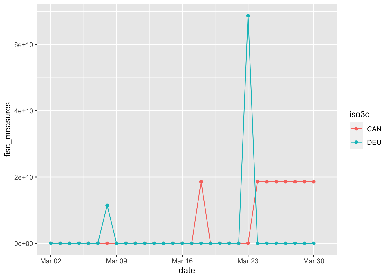
Summary
I applaud the Oxford team for crowd-sourcing such an impressive dataset in such a short period of time. However, given the current status of the data, I cannot advise to use the financial measurement data.
The main data, the policy measures, seem to be in better shape. Nevertheless, also these items do not come without issues. The organization in wide format creates redundant data and introduces as well as conceals potential coding errors. The distinction between zero and missing values is unclear. Later days in March sometimes have missing values. The calculation of the Stringency Index is not described in sufficient detail to warrant effortless reproduction. While generally, policy measures are coded as levels it appears as if in some cases they are coded as interventions instead. The notes to the policy measures could be more authoritative.
Compared to the Oxford data, the ACAPS data spans more countries, has more observations, finer categories, provides also some information on the regional structure of interventions, comes in a tidier format and has more authoritative sources included. Comparing the measures provided by both data sources shows that, while both exhibit clearly similar patterns, country-level averages vary considerably. This implies that the choice of the data source might have an impact on research findings.
My hope is that this review is helpful in improving the integrity of these important data sources as high quality data on non-pharmaceutical interventions will be instrumental to assess their effects going forward.
