Tidying the new Johns Hopkins Covid-19 time-series datasets

Pulling and tidying the Johns Hopkins Covid-19 data to long format at the country level

So here is the new code for pulling and tidying the data. After organizing everything by iso3c it merges the country names that are present in the Johns Hopkins data, giving prominence to the names that are present in the crurent datasets.

library(tidyverse)
library(lubridate)
library(countrycode)

clean_jhd_to_long <- function(df) {
  df_str <- deparse(substitute(df))
  var_str <- substr(df_str, 1, str_length(df_str) - 4)
  
  df %>% 
    select(-`Province/State`, -Lat, -Long) %>%
    rename(country = `Country/Region`) %>%
    mutate(iso3c = countrycode(country,
                               origin = "country.name",
                               destination = "iso3c")) %>%
    select(-country) %>%
    filter(!is.na(iso3c)) %>%
    group_by(iso3c) %>%
    summarise_at(vars(-group_cols()), sum) %>% 
    pivot_longer(
      -iso3c, 
      names_to = "date_str", 
      values_to = var_str
    ) %>%
    ungroup() %>%
    mutate(date = mdy(date_str)) %>%
    select(iso3c, date, !! sym(var_str)) 
}

confirmed_raw <- read_csv("https://raw.githubusercontent.com/CSSEGISandData/COVID-19/master/csse_covid_19_data/csse_covid_19_time_series/time_series_covid19_confirmed_global.csv", col_types = cols())
deaths_raw <- read_csv("https://raw.githubusercontent.com/CSSEGISandData/COVID-19/master/csse_covid_19_data/csse_covid_19_time_series/time_series_covid19_deaths_global.csv", col_types = cols())

# Recovered data I pull from the old depreciated dataset. This might generate issues going forward
recovered_raw <- read_csv("https://raw.githubusercontent.com/CSSEGISandData/COVID-19/master/csse_covid_19_data/csse_covid_19_time_series/time_series_19-covid-Recovered.csv", col_types = cols())

jh_covid19_data <- clean_jhd_to_long(confirmed_raw) %>%
  full_join(clean_jhd_to_long(deaths_raw), by = c("iso3c", "date")) %>%
  full_join(clean_jhd_to_long(recovered_raw), by = c("iso3c", "date"))

jhd_countries <- tibble(
  country = unique(confirmed_raw$`Country/Region`),
  iso3c = countrycode(country,
                      origin = "country.name",
                      destination = "iso3c")
) %>% filter(!is.na(iso3c))

old_jhd_countries <- tibble(
  country = unique(recovered_raw$`Country/Region`),
  iso3c = countrycode(country,
                      origin = "country.name",
                      destination = "iso3c")
) %>% filter(!is.na(iso3c),
             ! iso3c %in% jhd_countries$iso3c)

jhd_countries <- rbind(jhd_countries, old_jhd_countries)

jh_covid19_data %>%
  left_join(jhd_countries, by = "iso3c") %>%
  select(country, iso3c, date, confirmed, deaths, recovered) -> jh_covid19_data

# write_csv(jh_covid19_data, sprintf("jh_covid19_data_%s.csv", Sys.Date()))

Merging some World Bank data

The next code snippet pulls some World Bank data using the {wbstats} package.

library(tidyverse)
library(wbstats)

pull_worldbank_data <- function(vars) {
  new_cache <- wbcache()
  all_vars <- as.character(unique(new_cache$indicators$indicatorID))
  data_wide <- wb(indicator = vars, mrv = 10, return_wide = TRUE)
  new_cache$indicators[new_cache$indicators[,"indicatorID"] %in% vars, ] %>%
    rename(var_name = indicatorID) %>%
    mutate(var_def = paste(indicator, "\nNote:",
                           indicatorDesc, "\nSource:", sourceOrg)) %>%
    select(var_name, var_def) -> wb_data_def
  new_cache$countries %>%
    select(iso3c, iso2c, country, region, income) -> ctries
  left_join(data_wide, ctries, by = "iso3c") %>%
    rename(year = date,
           iso2c = iso2c.y,
           country = country.y) %>%
    select(iso3c, iso2c, country, region, income, everything()) %>%
    select(-iso2c.x, -country.x) %>%
    filter(!is.na(NY.GDP.PCAP.KD),
           region != "Aggregates") -> wb_data
  wb_data$year <- as.numeric(wb_data$year)
  wb_data_def<- left_join(data.frame(var_name = names(wb_data),
                                     stringsAsFactors = FALSE),
                          wb_data_def, by = "var_name")
  wb_data_def$var_def[1:6] <- c(
    "Three letter ISO country code as used by World Bank",
    "Two letter ISO country code as used by World Bank",
    "Country name as used by World Bank",
    "World Bank regional country classification",
    "World Bank income group classification",
    "Calendar year of observation"
  )
  wb_data_def$type = c("cs_id", rep("factor",  4), "ts_id",
                       rep("numeric", ncol(wb_data) - 6))
  return(list(wb_data, wb_data_def))
}

vars <- c("SP.POP.TOTL", "AG.LND.TOTL.K2", "EN.POP.DNST", "EN.URB.LCTY", "SP.DYN.LE00.IN", "NY.GDP.PCAP.KD")
wb_list <- pull_worldbank_data(vars)
wb_data <- wb_list[[1]]
wb_data_def <- wb_list[[2]]

wb_data %>%
  group_by(iso3c) %>%
  arrange(iso3c, year) %>%
  summarise(
    population = last(na.omit(SP.POP.TOTL)),
    land_area_skm = last(na.omit(AG.LND.TOTL.K2)),
    pop_density = last(na.omit(EN.POP.DNST)),
    pop_largest_city = last(na.omit(EN.URB.LCTY)),
    gdp_capita = last(na.omit(NY.GDP.PCAP.KD)),
    life_expectancy = last(na.omit(SP.DYN.LE00.IN))
  ) %>% left_join(wb_data %>% select(iso3c, region, income) %>% distinct()) -> wb_cs

# write_csv(wb_cs, "jh_add_wbank_data.csv")

suppressPackageStartupMessages({
  library(tidyverse)
  library(lubridate)
  library(gghighlight)
  library(ggrepel)
})

## Warning: package 'ggplot2' was built under R version 3.6.2

## Warning: package 'tibble' was built under R version 3.6.2

## Warning: package 'tidyr' was built under R version 3.6.2

## Warning: package 'readr' was built under R version 3.6.2

## Warning: package 'purrr' was built under R version 3.6.2

## Warning: package 'dplyr' was built under R version 3.6.2

## Warning: package 'lubridate' was built under R version 3.6.2

dta <- read_csv(
  "https://joachim-gassen.github.io/data/jh_covid19_data_2020-03-25.csv",
  col_types = cols()
) %>%
  mutate(date = ymd(date))

wb_cs <- read_csv(
  "https://joachim-gassen.github.io/data/jh_add_wbank_data.csv", 
  col_types = cols()
)

# I define event time zero where, for a given country, the confirmed
# cases match or exceed the Chinese case number at the beginning of the
# data so that all countries can be compared across event time.
# Also a require each country to have at least 7 days post event day 0

dta %>% 
  group_by(country) %>%
  filter(confirmed >= min(dta$confirmed[dta$country == "China"])) %>%
  summarise(edate_confirmed = min(date)) -> edates_confirmed

## `summarise()` ungrouping output (override with `.groups` argument)

dta %>% 
  left_join(edates_confirmed, by = "country") %>%
  mutate(
    edate_confirmed = as.numeric(date - edate_confirmed)
  ) %>%
  filter(edate_confirmed >= 0) %>%
  group_by(country) %>%
  filter (n() >= 7) %>% 
  ungroup() %>%
  left_join(wb_cs, by = "iso3c") %>% 
  mutate(
    confirmed_1e5pop = 1e5*confirmed/population
  ) -> df

lab_notes <- paste0(
  "Data as provided by Johns Hopkins University Center for Systems Science ", 
  "and Engineering (JHU CSSE)\nand obtained on March 23, 2020. ",
  "The sample is limited to countries with at least seven days of positive\n", 
  "event days data. Code and walk-through: https://joachim-gassen.github.io."
)

lab_x_axis_confirmed <- sprintf(paste(
  "Days since confirmed cases matched or exceeded\n", 
  "initial value reported for China (%d cases)\n"
), min(dta$confirmed[dta$country == "China"]))

gg_my_blob <- list(
  scale_y_continuous(trans='log10', labels = scales::comma),  
  theme_minimal(), 
  theme(
    plot.title.position = "plot", 
    plot.caption.position =  "plot",
    plot.caption = element_text(hjust = 0),
    axis.title.x = element_text(hjust = 1),
    axis.title.y = element_text(hjust = 1),
  ),
  labs(caption = lab_notes,
       x = lab_x_axis_confirmed,
       y = "Confirmed cases (logarithmic scale)"),
  gghighlight(TRUE,  label_key = country, use_direct_label = TRUE,
              label_params = list(segment.color = NA, nudge_x = 1))
)

ggplot(df %>% filter (edate_confirmed <= 30), 
       aes(x = edate_confirmed, color = country, y = confirmed)) +
  geom_line() +
  labs(
    title = "Focus on the first month: Confirmed Cases\n"
  ) +
  gg_my_blob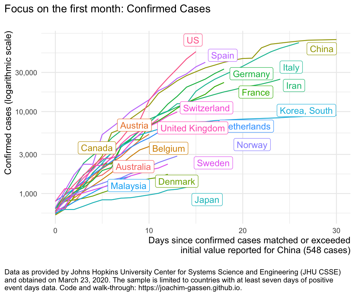

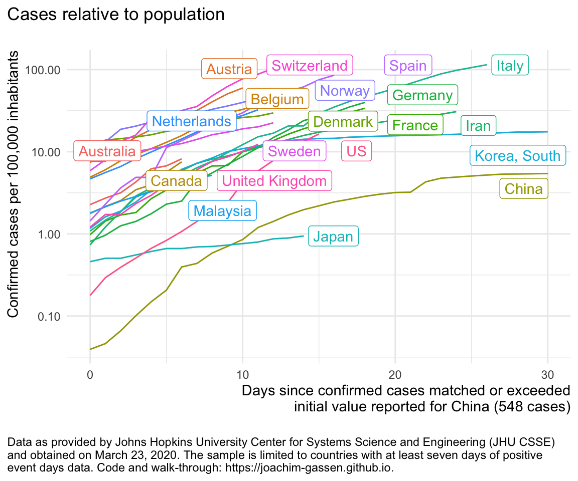
ggplot(df %>% filter (edate_confirmed <= 30), 
       aes(x = edate_confirmed, color = country, y = confirmed_1e5pop)) +
  geom_line() +
  gg_my_blob +
  labs(
    y = "Confirmed cases per 100,000 inhabitants",
    title = "Cases relative to population\n"
  ) 

Wrap-Up

This is it. I hope that somebody might fight this useful. In any case, help #FlattenTheCurve and stay healthy, everybody!

Appendix: Old code if you are interested in fuzzy matching

This is here for documentation purposes only. I would use the new code if I were you as it can be expected to be more robust moving forward.

library(tidyverse)
library(lubridate)
library(rvest)
library(stringdist)

# Function to read the raw CSV files. The files are aggregated to the country
# level and then converted to long format

clean_jhd_to_long <- function(df) {
  df_str <- deparse(substitute(df))
  var_str <- substr(df_str, 1, str_length(df_str) - 4)
  
  df %>% group_by(`Country/Region`) %>%
    filter(`Country/Region` != "Cruise Ship") %>%
    select(-`Province/State`, -Lat, -Long) %>%
    mutate_at(vars(-group_cols()), sum) %>% 
    distinct() %>%
    ungroup() %>%
    rename(country = `Country/Region`) %>%
    pivot_longer(
      -country, 
      names_to = "date_str", 
      values_to = var_str
    ) %>%
    mutate(date = mdy(date_str)) %>%
    select(country, date, !! sym(var_str)) 
}

confirmed_raw <- read_csv("https://raw.githubusercontent.com/CSSEGISandData/COVID-19/master/csse_covid_19_data/csse_covid_19_time_series/time_series_covid19_confirmed_global.csv")
deaths_raw <- read_csv("https://raw.githubusercontent.com/CSSEGISandData/COVID-19/master/csse_covid_19_data/csse_covid_19_time_series/time_series_covid19_deaths_global.csv")


jh_covid19_data <- clean_jhd_to_long(confirmed_raw) %>%
  full_join(clean_jhd_to_long(deaths_raw))


# Next, I pull official country level indicators from the UN Statstics Division
# to get country level identifiers.

jhd_countries <- tibble(country = unique(jh_covid19_data$country)) %>% arrange(country)

ctry_ids <- read_html("https://unstats.un.org/unsd/methodology/m49/") %>%
  html_table()
un_m49 <- ctry_ids[[1]]
colnames(un_m49) <- c("country", "un_m49", "iso3c")


# Merging by country name is messy. I start with a fuzzy matching approach
# using the {stringdist} package

ctry_names_dist <- matrix(NA, nrow = nrow(jhd_countries), ncol = nrow(un_m49))
for(i in 1:length(jhd_countries$country)) {
  for(j in 1:length(un_m49$country)) { 
    ctry_names_dist[i,j]<-stringdist(tolower(jhd_countries$country[i]), 
                                tolower(un_m49$country[j]))      
  }  
}

min_ctry_name_dist <- apply(ctry_names_dist, 1, min)

matched_ctry_names <- NULL

for(i in 1:nrow(jhd_countries)) {
  un_m49_row <- match(min_ctry_name_dist[i], ctry_names_dist[i,])
  if (length(which(ctry_names_dist[i,] %in% min_ctry_name_dist[i])) > 1) un_m49_row <- NA
  matched_ctry_names <- rbind(matched_ctry_names,
                         tibble( 
                           jhd_countries_row = i, 
                           un_m49_row = un_m49_row,
                           jhd_ctry_name = jhd_countries$country[i], 
                           un_m49_name = ifelse(is.na(un_m49_row), NA, 
                                                un_m49$country[un_m49_row])
                         ))
}

# This matches most cases well but some cases need to be adjusted by hand.
# In addition there are two jurisdictions (Kosovo, Taiwan)
# that cannot be matched as they are no 'country' as far as the U.N.
# Statistics Devision is concerned.

# WATCH OUT: The data from JHU is subject to change without notice.
# New countries are being added and names/spelling might change. 
# Also, in the long run, the data provided by the UNSD might change.
# Inspect 'matched_ctry_names' before using the data.

matched_ctry_names$un_m49_row[matched_ctry_names$jhd_ctry_name == "Bolivia"] <- 27
matched_ctry_names$un_m49_row[matched_ctry_names$jhd_ctry_name == "Brunei"] <- 35
matched_ctry_names$un_m49_row[matched_ctry_names$jhd_ctry_name == "Congo (Brazzaville)"] <- 54
matched_ctry_names$un_m49_row[matched_ctry_names$jhd_ctry_name == "Congo (Kinshasa)"] <- 64
matched_ctry_names$un_m49_row[matched_ctry_names$jhd_ctry_name == "East Timor"] <- 222
matched_ctry_names$un_m49_row[matched_ctry_names$jhd_ctry_name == "Iran"] <- 109
matched_ctry_names$un_m49_row[matched_ctry_names$jhd_ctry_name == "Korea, South"] <- 180
matched_ctry_names$un_m49_row[matched_ctry_names$jhd_ctry_name == "Kosovo"] <- NA
matched_ctry_names$un_m49_row[matched_ctry_names$jhd_ctry_name == "Moldova"] <- 181
matched_ctry_names$un_m49_row[matched_ctry_names$jhd_ctry_name == "Russia"] <- 184
matched_ctry_names$un_m49_row[matched_ctry_names$jhd_ctry_name == "Taiwan*"] <- NA
matched_ctry_names$un_m49_row[matched_ctry_names$jhd_ctry_name == "Tanzania"] <- 236
matched_ctry_names$un_m49_row[matched_ctry_names$jhd_ctry_name == "United Kingdom"] <- 235
matched_ctry_names$un_m49_row[matched_ctry_names$jhd_ctry_name == "US"] <- 238
matched_ctry_names$un_m49_row[matched_ctry_names$jhd_ctry_name == "Venezuela"] <- 243

# Last Step: Match country identifier data and save file (commented out here)
jhd_countries %>% 
  left_join(matched_ctry_names %>% 
              select(jhd_ctry_name, un_m49_row), 
            by = c(country = "jhd_ctry_name")) %>%
  left_join(un_m49 %>% mutate(un_m49_row = row_number()), by = "un_m49_row") %>%
  rename(country = country.x) %>%
  select(country, iso3c)  -> jhd_countries

jh_covid19_data <- jh_covid19_data %>% left_join(jhd_countries) %>%
  select(country, iso3c, date, confirmed, deaths)
  
# write_csv(jh_covid19_data, sprintf("jh_covid19_data_%s.csv", Sys.Date()))

The code essentially follows the following steps

• Read the relevant CSV files for confirmed cases and casualties from the Github repository
• Aggregate the data at country level and discard data that is not required
• Scrape official country identifiers from the U.N. Statistics Division
• Fuzzy match these to the countries present in the JH data. Apply manual corrections that were correct based on the data pulled March 23, 2020 (check the match when you use this code later)
• Merge the identifiers with the longitudinal data and save the result as a tidy CSV file.