Explore your Researcher Degrees of Freedom
I am an applied economist working in the area of accounting and corporate transparency. I work with observational data a lot, meaning with data that is already available and not under my control. Whenever I set sails to design a test, there are a lot of decisions to take: Which sample should I use? What is the appropriate time frame? How do I define my dependent and independent variables? What is the functional relation that I expect between dependent and independent variables? Can I identify potential confounders? Can I measure them? How do I deal with extreme observations? …
Sometimes, theory provides clear guidance but, frankly, at least in the social sciences sometimes it does not. So, in my experience, we often resort to an ex ante specification and ex post verification exercise. We decide the above choices partly ad hoc and then later run more or less arbitrary alternatives to verify whether our main findings are robust to these alternative model specifications.
Careful researchers that we are, we then finally settle for a set of different research specifications that we report. Taken together, we hope, these model results provide a fair representation of our analyses and the underlying data. After extensive work-shopping and resulting iterations, we happily submit our work. Then the reviewers and editors come back to us, often asking us to run additional specifications in order to second guess the robustness of our findings. Sometimes the final outcome if favorable, sometimes it is not.
Is this the best that we can do? Is this an efficient process that motivates researchers to provide fairly balanced views of their findings and editors to publish these views? Many prominent scholars from various fields have voiced their doubts. The problem has been coined as “Researcher Degrees of Freedom” by Simmons, Nelson and Simmonsohn or the “Garden of Forking Paths” by Gelman and Loken. In this blog post, I introduce the in-development R package rdfanaylsis that I develop to provide a hands-on coding environment that allows researchers to specify their researcher degrees of freedom ex ante and to systematically explore their effects on their findings ex post. The resulting code is self-documenting, and supports unit testing based on simulated data that can also be used to assess the consistency and power of a research design prior to taking it to the real data.
Explaining the inner workings of the package is beyond the scope of this blog post and I encourage the interested reader to take a look the package’s vignette if she is interested to take the package for a spin. In this post I will use some of the findings from the vignette to hopefully communicate the basic idea of the package.
I use a prominent topic from health economics and demographics to illustrate my point. Consider yourself concerned with measuring the effect of national income on life expectancy. There is a long ongoing debate about the existence and magnitude of this effect (see Lutz and Kebede, Pop and Dev Review 2018 for a recent contribution). Traditionally, you would collect data (in our case a country-year panel from the World Bank and the Wittgenstein Center), specify a suitable model and report your findings along with some robustness tests. A potential key table of a conventional study could look like the one below.
library(tidyverse)
library(ExPanDaR)
library(rdfanalysis)

res <- read_csv("https://joachim-gassen.github.io/data/wb_new.csv", col_types = cols()) %>%
  mutate_at(c("country", "year"), as.factor) %>%
  mutate_at(c("lifeexpectancy", "gdp_capita",
           "mn_yrs_school", "unemployment"), list(ln = log)) %>%
  select(country, region, year,
         gdp_capita, lifeexpectancy,
         mn_yrs_school, unemployment,
         gdp_capita_ln, lifeexpectancy_ln,
         mn_yrs_school_ln, unemployment_ln) %>%
  na.omit() %>%
  treat_outliers(percentile = 0.01) %>%
  prepare_regression_table(dvs = rep("lifeexpectancy", 6),
                           idvs = list(c("gdp_capita_ln", "mn_yrs_school_ln", "unemployment_ln"),
                                       c("gdp_capita_ln"),
                                       c("gdp_capita", "mn_yrs_school", "unemployment"),
                                       c("gdp_capita_ln", "mn_yrs_school_ln", "unemployment_ln"),
                                       c("gdp_capita_ln", "mn_yrs_school_ln", "unemployment_ln"),
                                       c("gdp_capita_ln", "mn_yrs_school_ln", "unemployment_ln")),
                           feffects = list(c("country", "year"), c("country", "year"),
                                           c("country", "year"), "country", "year", ""),
                           clusters = list(c("country", "year"), c("country", "year"),
                                           c("country", "year"), "country", "year", ""))

htmltools::HTML(res$table)| Dependent variable: | ||||||
| lifeexpectancy | lifeexpectancy | lifeexpectancy | lifeexpectancy | lifeexpectancy | lifeexpectancy | |
| (1) | (2) | (3) | (4) | (5) | (6) | |
| gdp_capita_ln | 1.241*** | 1.096*** | 3.014*** | 3.481*** | 3.448*** | |
| (0.405) | (0.372) | (0.613) | (0.029) | (0.079) | ||
| mn_yrs_school_ln | 7.499*** | 13.270*** | 6.315*** | 6.773*** | ||
| (1.299) | (1.121) | (0.130) | (0.234) | |||
| unemployment_ln | -0.148 | -0.300 | -0.465*** | -0.563*** | ||
| (0.338) | (0.347) | (0.060) | (0.106) | |||
| gdp_capita | -0.0001* | |||||
| (0.00004) | ||||||
| mn_yrs_school | 0.543 | |||||
| (0.447) | ||||||
| unemployment | -0.071* | |||||
| (0.041) | ||||||
| Constant | 27.160*** | |||||
| (0.477) | ||||||
| Estimator | ols | ols | ols | ols | ols | ols |
| Fixed effects | country, year | country, year | country, year | country | year | None |
| Std. errors clustered | country, year | country, year | country, year | country | year | No |
| Observations | 3,998 | 3,998 | 3,998 | 3,998 | 3,998 | 3,998 |
| R2 | 0.975 | 0.972 | 0.972 | 0.970 | 0.718 | 0.708 |
| Adjusted R2 | 0.974 | 0.970 | 0.971 | 0.969 | 0.716 | 0.707 |
| Note: | *p<0.1; **p<0.05; ***p<0.01 | |||||
This table communicates a fairly robust association of our measure for national income (gross domestic production per inhabitant, GDP per capita) with life expectancy. In terms of economic magnitude, the coefficients translate into an effect of a 10 % increase in GDP on life expectancy of roughly 2.5 * log(1.1) = 0.24 years, where the factor 2.5 is based on the average of the log-transformed GDP per capita coefficients.
Obviously, this research design has some inherent choices. Why did I delete missing observations prior to winsorizing? Why did I winsorize the data? Why did I report univariate and multi-variate findings but no findings with just one additional control variable? Why do I present level-log and level-level models but no log-log or log-level models? How did I decide on fixed effect structures and the clustering of the standard errors? The list goes on and on.
The rdfanalysis package provides me with an infrastructure to systematically document and explore these researcher degrees of freedom. As a first step, after documenting the research design and its choices in code, a function of the package parses the code to generate a quick visualization of the design. For our problem at hand, it generates the following (see vignette of package for code of all what follows).
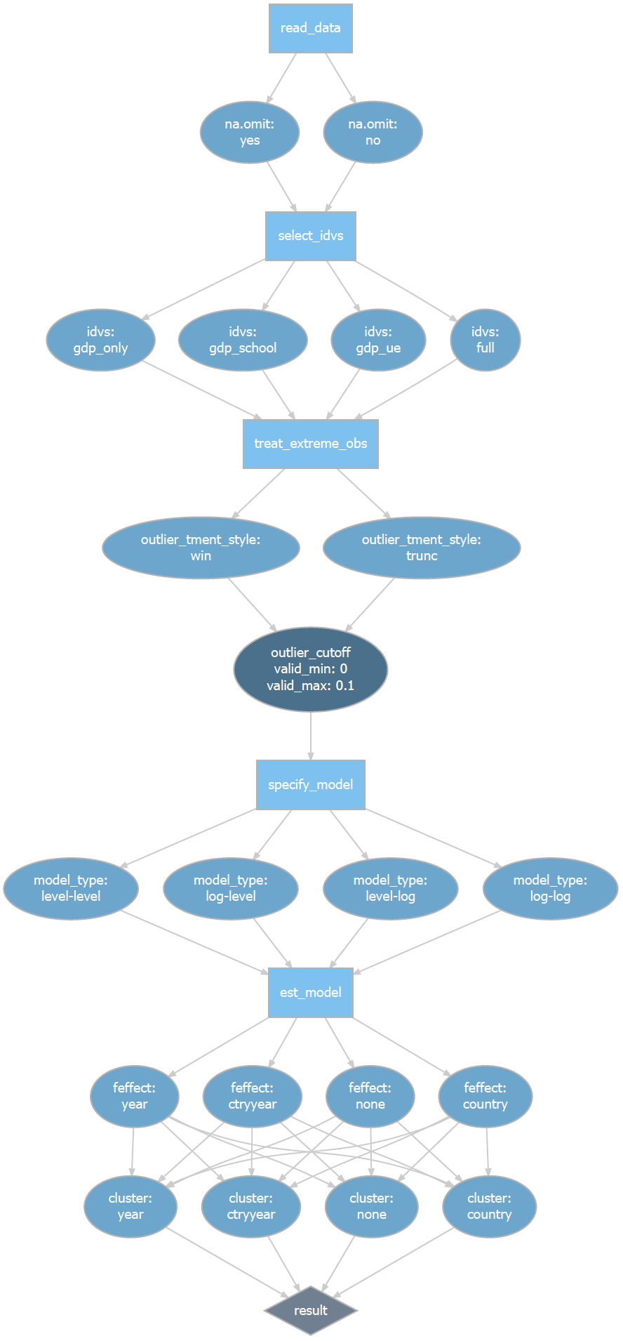
Research Design Flow with Degrees of Freedom Paths
Try to guess the number of paths (referred to as protocols within the rdfanalysis package) that you could take through this rather simplistic test design! In principle, the number is infinite because of the continuous choice of the outlier cut-off but when you restrict this choice to percentiles this design represents you with a whooping number of 11,264 degrees of freedom!
The beauty of the rdfanaylsis package it that it allows you to exhaust your analysis across all feasible protocols with a single command. More explicitly, I propose the following workflow which outlines the structure of the rdfanalysis package:
- Develop your design by identifying the necessary steps and specifying as well as implementing all choices for each step.
- Pre-specify the protocols that you hypothesize to be most supported by theory by assigning weights to them. This should be done prior to working with real data.
- Use simulated data and your pre-assigned weights to verify that your implementation produces findings consistent with your identifying assumptions and assess the power of your design.
- Run your design on your real data, producing all estimates with positive weights. The weighted mean estimate and its confidence interval constitutes your test result.1
- Run your design across all feasible choices to assess the robustness of your finding relative to choosing alternative protocols.
For the problem at hand, I let theory and intuition guide me to decide that 12 protocols should have positive weights to generate my test results. To compare effect sizes across different model specifications, I re-calibrated coefficients so that my results always specify the effect of a 10 % increase in GDP per capita on life expectancy in years. Here are my 12 model results as stored by rdfanalysis (again, refer to the vignette to see how the loaded data is being generated):
load("../../static/data/rdf_ests.RData")
kable(weighted_ests, digits = 3)| na.omit | idvs | outlier_tment_style | outlier_cutoff | model_type | feffect | cluster | weight | est | lb | ub |
|---|---|---|---|---|---|---|---|---|---|---|
| yes | full | win | 0.00 | level-log | ctryyear | ctryyear | 0.05 | 0.136 | 0.046 | 0.225 |
| yes | full | trunc | 0.00 | level-log | ctryyear | ctryyear | 0.05 | 0.136 | 0.046 | 0.225 |
| yes | full | win | 0.01 | level-log | ctryyear | ctryyear | 0.10 | 0.118 | 0.041 | 0.196 |
| yes | full | trunc | 0.01 | level-log | ctryyear | ctryyear | 0.10 | 0.104 | 0.036 | 0.173 |
| yes | full | win | 0.05 | level-log | ctryyear | ctryyear | 0.10 | 0.095 | 0.024 | 0.167 |
| yes | full | trunc | 0.05 | level-log | ctryyear | ctryyear | 0.10 | 0.079 | 0.006 | 0.152 |
| yes | full | win | 0.00 | log-log | ctryyear | ctryyear | 0.05 | 0.164 | 0.053 | 0.274 |
| yes | full | trunc | 0.00 | log-log | ctryyear | ctryyear | 0.05 | 0.164 | 0.053 | 0.274 |
| yes | full | win | 0.01 | log-log | ctryyear | ctryyear | 0.10 | 0.135 | 0.047 | 0.223 |
| yes | full | trunc | 0.01 | log-log | ctryyear | ctryyear | 0.10 | 0.116 | 0.043 | 0.190 |
| yes | full | win | 0.05 | log-log | ctryyear | ctryyear | 0.10 | 0.093 | 0.013 | 0.174 |
| yes | full | trunc | 0.05 | log-log | ctryyear | ctryyear | 0.10 | 0.083 | 0.007 | 0.160 |
The weighted mean estimate of these twelve models is 0.12 years with a confidence interval ranging from 0.03 to 0.19 years. This does not include my average estimate of 0.24 years from the conventional analysis above! Let’s look at the robustness of this estimate by exhausting all researcher degrees of freedom.
plot_rdf_estimate_density(ests, "est", "lb", "ub", color = "lightblue") +
  theme_minimal()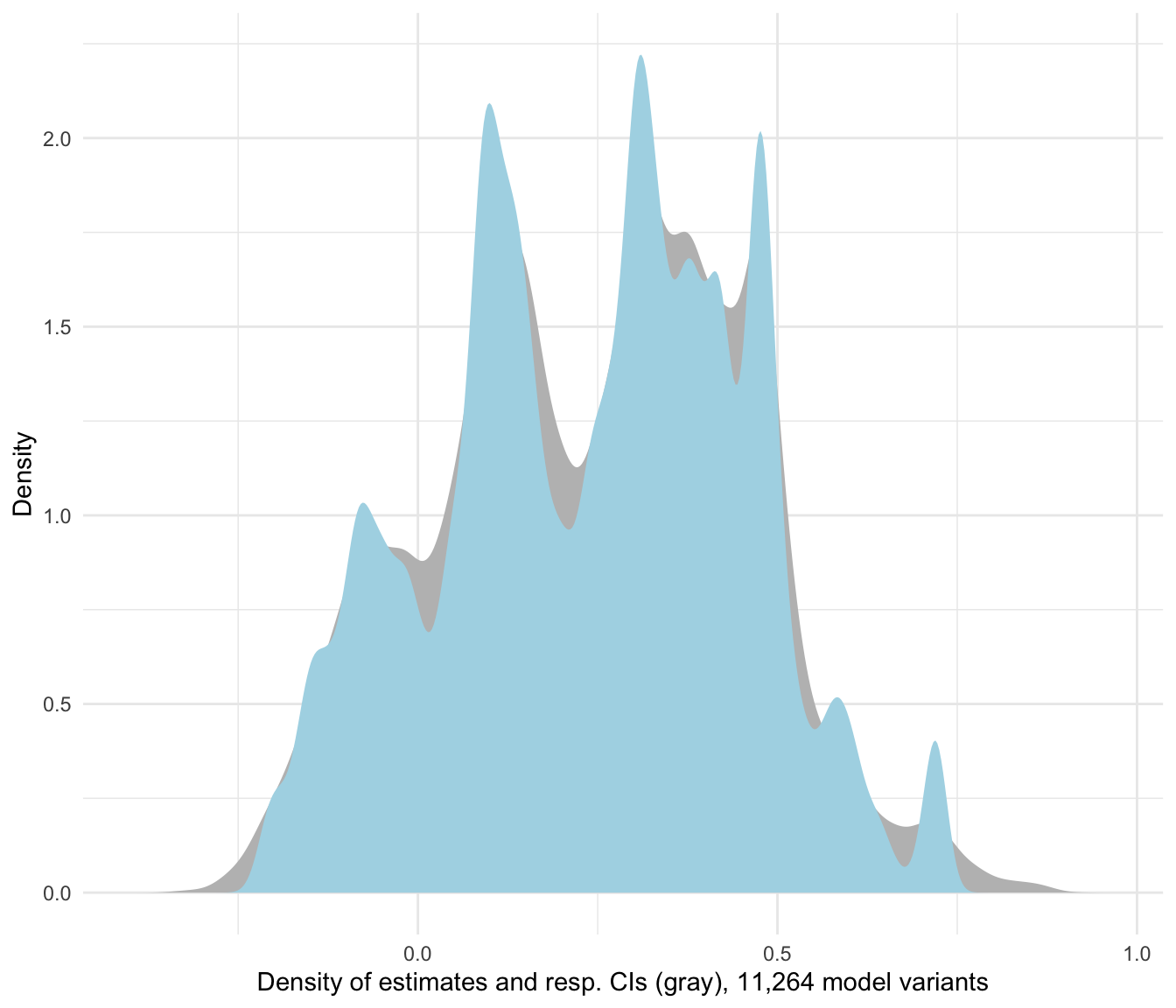
Figure 1: Estimate density for all researcher degrees of freedom
Now this provides quite a range of estimates, ranging from -0.35 to 0.92 years! To understand why the estimates vary across protocols, rdfanalysis provides some simple helper functions to generate visual displays of the data. For example, to see the impact of the fixed effect structure on the findings:
plot_rdf_ridges_by_dchoice(ests, "est", "feffect", hist = TRUE,
                           scale = 0.9, fill = "lightblue", color = NA)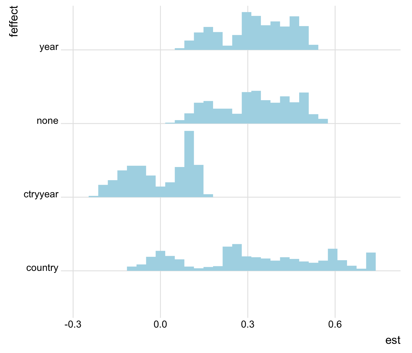
Figure 2: Estimates by fixed effect structure
Or, to see how the model specification affects the findings:
plot_rdf_ridges_by_dchoice(ests, "est", "model_type", hist = TRUE,
                           scale = 0.9, fill = "lightblue", color = NA)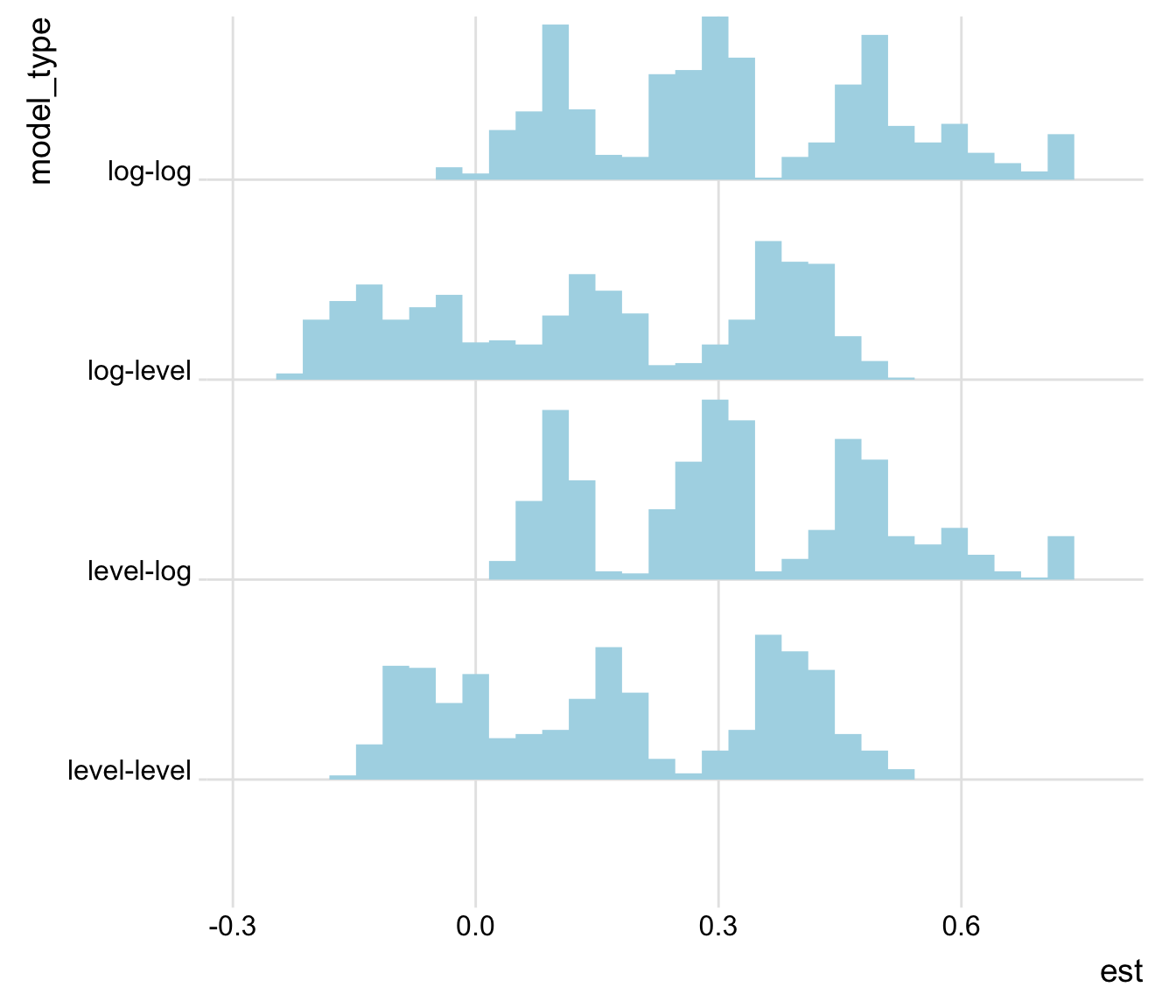
Figure 3: Estimates by model specification
You can drill down to the single protocol level by limiting your analysis on certain dimensions. As an example: Below you see a visual that displays how outlier treatments affect the findings of models based on the sparse sample, log-transformed independent variables, country and year fixed effects and two-way clustered standard errors that include only GDP per capita and years of schooling as independent variables.
ests %>%
  filter(na.omit == "no",
         idvs == "gdp_school",
         model_type == "level-log" | model_type == "log-log",
         feffect == "ctryyear",
         cluster == "ctryyear") %>%
  plot_rdf_estimates_by_choice("est", "lb", "ub", "outlier_tment_style",
                               color = "model_type", order = "outlier_cutoff", width = 0.008)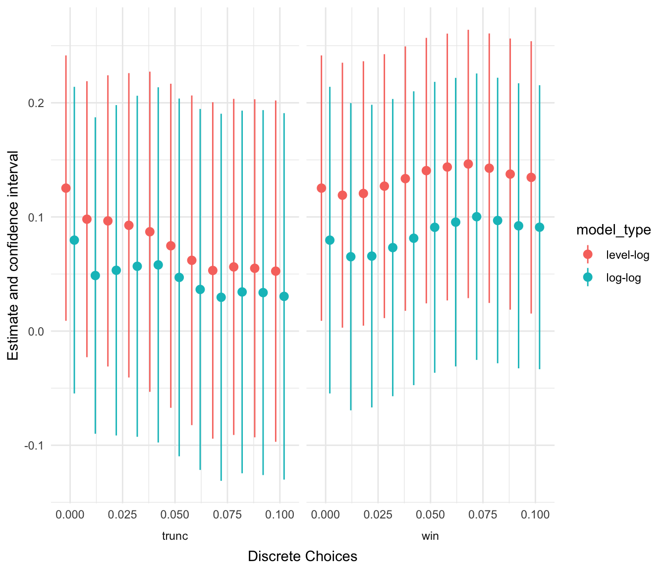
Figure 4: Outlier effects
Compare these insights about the robustness of our estimate to the insights that you can obtain from traditional robustness sections. I hope that you agree with me that there is an improvement.
By the way, if you are more of the “see-for-yourself playful” type, this kind of analysis can be accompanied by tools for interactive data and results exploration. See here for an example that allows you to explore the underlying data and re-construct the protocols of this analysis on the fly. The shiny app is based on another project of mine, the ExPanDaR package.
Taken together, I hope that these tools will help us make our findings more insightful. If you have remarks about the rdfanalysis package or this project in general, I would love to hear from you. Feel free to comment below. Alternatively, you can reach me via email or twitter.
Enjoy!
Conditional on the structure of the problem at hand, one can do much better in combining the insights from the different protocols than just generating a weighted average of their estimates. The literature on “model averaging” provides useful pointers.↩
